47 Discussion 07: BN Inference and Sampling (From Spring 2025)
In a Bayesian network, rather than storing information in a giant table, probabilities are instead distributed across a large number of smaller local probability tables along with a directed acyclic graph (DAG) which captures the relationships between variables. Thus, if we have a node representing variable \(X\), we store \(P(X \mid A_1, A_2, \ldots, A_N)\), where \(A_1, \ldots, A_N\) are the parents of \(X\).
- Each node is conditionally independent of all its ancestor nodes (non-descendants) in the graph, given all of its parents.
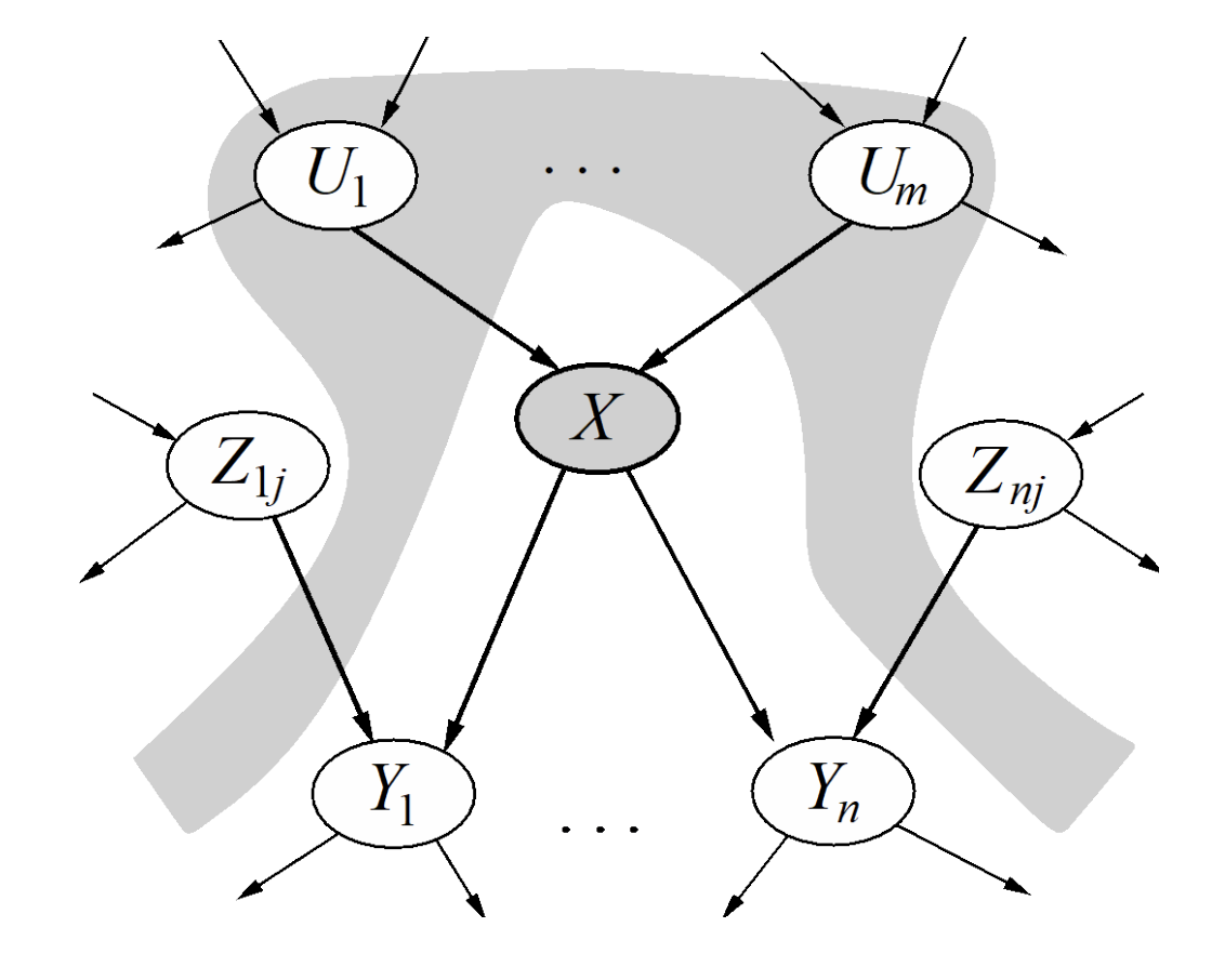
- Each node is conditionally independent of all other variables given its Markov blanket.
A variable’s Markov blanket consists of parents, children, and children’s other parents.
An alternate approach to inference by enumeration, where we eliminate variables one by one in order to reduce the maximum size of any factor generated.
Suppose we have the following Bayes Net with factors \(P(T)\), \(P(C|T)\), \(P(S|T)\), and \(P(E|C, S)\), and we want to compute \(P(T| + e)\).
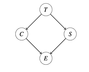
We proceed by eliminating the variables \(C\) and \(S\):
- Join (multiply) all the factors involving \(C\), forming \(P(C, +e|T, S) = P(C|T) · P(+e|C, S)\).
- Sum out C from this new factor, leaving us with a new factor \(P(+e|T, S)\).
- Join all factors involving \(S\), forming \(P(+e, S|T) = P(S|T) · P(+e|T, S)\).
- Sum out \(S\), yielding \(P(+e|T)\).
- Join the remaining two factors \(P(T)\) and \(P(+e|T)\) and normalize to get \(P(T| + e)\).
Suppose we want to evaluate \(P(Q \mid E)\) where \(Q\) are the query variables and \(E\) are the evidence variables.
Prior Sampling: Draw samples from the Bayes net by sampling the parents and then sampling the children given the parents.
\(P(Q \mid E) \approx \dfrac{\text{count}(Q \text{ and } E)}{\text{count}(E)}\).
Rejection Sampling: Like prior sampling, but ignore all samples that are inconsistent with the evidence.
Likelihood Weighting: Fix the evidence variables, and weight each sample by the probability of the evidence variables given their parents.
Gibbs Sampling:
- Fix evidence.
- Initialize other variables randomly.
- Repeat:
- Choose non-evidence variable \(X\).
- Resample \(X\) from \(P(X \mid \text{Markov blanket}(X))\)
- Choose non-evidence variable \(X\).
47.1 Variable Elimination
Using the same Bayes Net (shown below), we want to compute \(P(Y \mid +z)\).
All variables have binary domains. Assume we run variable elimination to compute the answer to this query, with the following variable elimination ordering: \(X, T, U, V, W\).
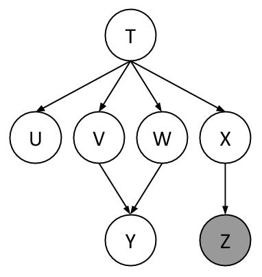
After inserting evidence, we have the following factors to start out with:
\[ P(T), \; P(U \mid T), \; P(V \mid T), \; P(W \mid T), \; P(X \mid T), \; P(Y \mid V,W), \; P(+z \mid X) \]
47.1.1 (a)
When eliminating \(X\) we generate a new factor \(f_1\) as follows, which leaves us with the factors:
Answer
\[ f_1(+z \mid T) = \sum_x P(x \mid T) P(+z \mid x) \]
Resulting factors:\[ P(T), \; P(U \mid T), \; P(V \mid T), \; P(W \mid T), \; P(Y \mid V,W), \; f_1(+z \mid T) \]
47.1.2 (b)
When eliminating \(T\) we generate a new factor \(f_2\) as follows, which leaves us with the factors:
Answer
\[ f_2(U,V,W,+z) = \sum_t P(t) P(U \mid t) P(V \mid t) P(W \mid t) f_1(+z \mid t) \]
Resulting factors:\[ P(Y \mid V,W), \; f_2(U,V,W,+z) \]
47.1.3 (c)
When eliminating \(U\) we generate a new factor \(f_3\) as follows, which leaves us with the factors:
Answer
\[ f_3(V,W,+z) = \sum_u f_2(u,V,W,+z) \]
Resulting factors:
\[
P(Y \mid V,W), \; f_3(V,W,+z)
\]
\(\sum_u P(U \mid t) = 1\). We can see this in the graph: we can remove any leaf node that is not a query variable or an evidence variable.
47.1.4 (d)
When eliminating \(V\) we generate a new factor \(f_4\) as follows, which leaves us with the factors:
Answer
\[ f_4(W,Y,+z) = \sum_v f_3(v,W,+z) P(Y \mid v,W) \]
Resulting factors:\[ f_4(W,Y,+z) \]
47.1.5 (e)
When eliminating \(W\) we generate a new factor \(f_5\) as follows, which leaves us with the factors:
Answer
\[ f_5(Y,+z) = \sum_w f_4(w,Y,+z) \]
Resulting factors:\[ f_5(Y,+z) \]
47.1.6 (f)
How would you obtain \(P(Y \mid +z)\) from the factors left above?
Answer
Simply renormalize \(f_5(Y,+z)\) to obtain \(P(Y \mid +z)\):
\[ P(y \mid +z) = \frac{f_5(y,+z)}{\sum_{y'} f_5(y',+z)} \]47.1.7 (g)
What is the size of the largest factor that gets generated during the above process?
Answer
The largest factor is:
\[
f_2(U,V,W,+z)
\]
(\(U, V, W\) are binary variables, and we only need to store the probability for \(+z\) for each possible setting of these variables).
47.1.8 (h)
Does there exist a better elimination ordering (one which generates smaller largest factors)?
Answer
Yes. One such ordering is:
\[
X, U, T, V, W
\]
47.2 Bayes’ Nets Sampling
Assume the following Bayes’ net, and the corresponding distributions over the variables in the Bayes’ net:
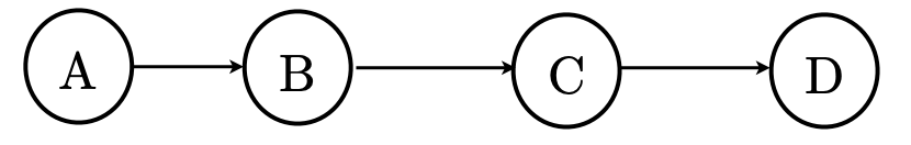
| \(P(A)\) | |
|---|---|
| \(-a\) | 3/4 |
| \(+a\) | 1/4 |
| \(P(B|A)\) | ||
|---|---|---|
| \(-a\) | \(-b\) | 2/3 |
| \(-a\) | \(+b\) | 1/3 |
| \(+a\) | \(-b\) | 4/5 |
| \(+a\) | \(+b\) | 1/5 |
| \(P(C|B)\) | ||
|---|---|---|
| \(-b\) | \(-c\) | 1/4 |
| \(-b\) | \(+c\) | 3/4 |
| \(+b\) | \(-c\) | 1/2 |
| \(+b\) | \(+c\) | 1/2 |
| \(P(D|C)\) | ||
|---|---|---|
| \(-c\) | \(-d\) | 1/8 |
| \(-c\) | \(+d\) | 7/8 |
| \(+c\) | \(-d\) | 5/6 |
| \(+c\) | \(+d\) | 1/6 |
47.2.1 (a)
You are given the following samples:
47.2.1.1 (i)
Assume that these samples came from performing Prior Sampling, and calculate the sample estimate of \(P(+c)\).
Answer
\(\frac{5}{8}\)47.2.1.2 (ii)
Now we will estimate \(P(+c | +a, −d)\). Above, clearly cross out the samples that would not be used when doing Rejection Sampling for this task, and write down the sample estimate of \(P(+c | +a, −d)\) below.
Answer
\(\frac{2}{3}\)
47.2.2 (b)
Using Likelihood Weighting Sampling to estimate \(P(−a | +b, −d)\), the following samples were obtained. Fill in the weight of each sample in the corresponding row.
| Sample | Weight |
|---|---|
| \(-a \; +b \; +c \; -d\) | |
| \(+a \; +b \; +c \; -d\) | |
| \(+a \; +b \; -c \; -d\) | |
| \(-a \; +b \; -c \; -d\) |
Answer
| Sample | Weight |
|---|---|
| \(-a,\; +b,\; +c,\; -d\) | \(P(+b \mid -a)\,P(-d \mid +c) = \tfrac{1}{3} \cdot \tfrac{5}{6} = \tfrac{5}{18} = 0.277\) |
| \(+a,\; +b,\; +c,\; -d\) | \(P(+b \mid +a)\,P(-d \mid +c) = \tfrac{1}{5} \cdot \tfrac{5}{6} = \tfrac{5}{30} = \tfrac{1}{6} = 0.17\) |
| \(+a,\; +b,\; -c,\; -d\) | \(P(+b \mid +a)\,P(-d \mid -c) = \tfrac{1}{5} \cdot \tfrac{1}{8} = \tfrac{1}{40} = 0.025\) |
| \(-a,\; +b,\; -c,\; -d\) | \(P(+b \mid -a)\,P(-d \mid -c) = \tfrac{1}{3} \cdot \tfrac{1}{8} = \tfrac{1}{24} = 0.042\) |
47.2.3 (c)
From the weighted samples in the previous question, estimate \(P(−a | +b, −d)\).
Answer
\[ \frac{5/18+1/24}{5/18+5/30+1/40+1/24} = 0.625 \]47.2.4 (d)
Which query is better suited for likelihood weighting, \(P(D | A)\) or \(P(A | D)\)? Justify your answer in one sentence.
Answer
\(P(D | A)\) is better suited for likelihood weighting sampling, because likelihood weighting conditions only on upstream evidence.47.2.5 (e)
Recall that during Gibbs Sampling, samples are generated through an iterative process.
Assume that the only evidence that is available is \(A = +a\). Clearly fill in the circle(s) of the sequence(s) below that could have been generated by Gibbs Sampling.
Sequence 1 \[ \begin{array}{r@{\,}c@{\,}c@{\,}c@{\,}c} \hline \text{1:} & +a & -b & -c & +d \\ \text{2:} & +a & -b & -c & +d \\ \text{3:} & +a & -b & +c & +d \\ \hline \end{array} \]
Sequence 2 \[ \begin{array}{r@{\,}c@{\,}c@{\,}c@{\,}c} \hline \text{1:} & +a & -b & -c & +d \\ \text{2:} & +a & -b & -c & -d \\ \text{3:} & -a & -b & -c & +d \\ \hline \end{array} \]
Sequence 3 \[ \begin{array}{r@{\,}c@{\,}c@{\,}c@{\,}c} \hline \text{1:} & +a & -b & -c & +d \\ \text{2:} & +a & -b & -c & -d \\ \text{3:} & +a & +b & -c & -d \\ \hline \end{array} \]
Sequence 4 \[ \begin{array}{r@{\,}c@{\,}c@{\,}c@{\,}c} \hline \text{1:} & +a & -b & -c & +d \\ \text{2:} & +a & -b & -c & -d \\ \text{3:} & +a & +b & -c & +d \\ \hline \end{array} \]
Answer
Gibbs sampling updates one variable at a time and never changes the evidence.
The first and third sequences have at most one variable change per row, and hence could have been generated from Gibbs sampling. In sequence 2, the evidence variable is changed. In sequence 4, the second and third samples have both \(B\) and \(D\) changing.