39  Discussion 11: ML II (From Spring 2025)

Slides

39.1 Optimization

We would like to classify some data. We have N samples, where each sample consists of a feature vector \(\mathbf{x} = [x_1, \cdots, x_k]^T \text{ and a label } y \in \{0, 1\}.\)

Logistic regression produces predictions as follows:

\[ P(Y=1|X) = h(\mathbf{x}) = s\left(\sum_i w_i x_i\right) = \frac{1}{1+\exp\left(-\left(\sum_i w_i x_i\right)\right)} \]

\[ s(\gamma) = \frac{1}{1+\exp(-\gamma)} \]

where \(s(\gamma)\) is the logistic function, \(\exp x = e^x\), and \(\mathbf{w} = [w_1, \cdots, w_k]^T\) are the learned weights.

Let’s find the weights \(w_j\) for logistic regression using stochastic gradient descent. We would like to minimize the following loss function (called the cross-entropy loss) for each sample:

\[ L = -[y \ln h(\mathbf{x}) + (1-y) \ln(1-h(\mathbf{x}))] \]

---

39.1.1 (a)

Show that \(s'(\gamma) = s(\gamma)(1-s(\gamma))\)

Answer

\[ \begin{aligned} s(\gamma) &= (1+\exp(-\gamma))^{-1} \\ s'(\gamma) &= -(1+\exp(-\gamma))^{-2}(-\exp(-\gamma)) \\ s'(\gamma) &= \frac{1}{1+\exp(-\gamma)} \cdot \frac{\exp(-\gamma)}{1+\exp(-\gamma)} \\ s'(\gamma) &= s(\gamma)(1-s(\gamma)) \end{aligned} \]

---

39.1.2 (b)

Find \(\frac{dL}{dw_j}\). Use the fact from the previous part.

Answer

Use chain rule: \[ \frac{dL}{dw_j} = -\left[\frac{y}{h(\mathbf{x})} s'\left(\sum_i w_i x_i\right)x_j - \frac{1-y}{1-h(\mathbf{x})} s'\left(\sum_i w_i x_i\right)x_j\right] \]

Use fact from previous part: \[ \frac{dL}{dw_j} = -\left[\frac{y}{h(\mathbf{x})} h(\mathbf{x})(1-h(\mathbf{x}))x_j - \frac{1-y}{1-h(\mathbf{x})} h(\mathbf{x})(1-h(\mathbf{x}))x_j\right] \]

Simplify: \[ \begin{aligned} \frac{dL}{dw_j} &= -[y(1-h(\mathbf{x}))x_j - (1-y)h(\mathbf{x})x_j] \\ &= -x_j[y-yh(\mathbf{x}) - h(\mathbf{x}) + yh(\mathbf{x})] \\ &= -x_j(y-h(\mathbf{x})) \end{aligned} \]

---

39.1.3 (c)

Now, find a simple expression for \(\nabla_{\mathbf{w}}L = \left[\frac{dL}{dw_1}, \frac{dL}{dw_2}, \dots, \frac{dL}{dw_k}\right]^T\)

Answer

\[ \begin{aligned} \nabla_{\mathbf{w}}L &= [-x_1(y-h(\mathbf{x})), -x_2(y-h(\mathbf{x})), \dots, -x_k(y-h(\mathbf{x}))]^T \\ &= - [x_1, x_2, \dots x_k]^T (y-h(\mathbf{x})) \\ &= -\mathbf{x}(y-h(\mathbf{x})) \end{aligned} \]

---

39.1.4 (d)

Write the stochastic gradient descent update for \(\mathbf{w}\). Our step size is \(\eta\).

Answer

\[ \mathbf{w} \leftarrow \mathbf{w} + \eta\mathbf{x}(y-h(\mathbf{x})) \]

39.2 Neural Nets

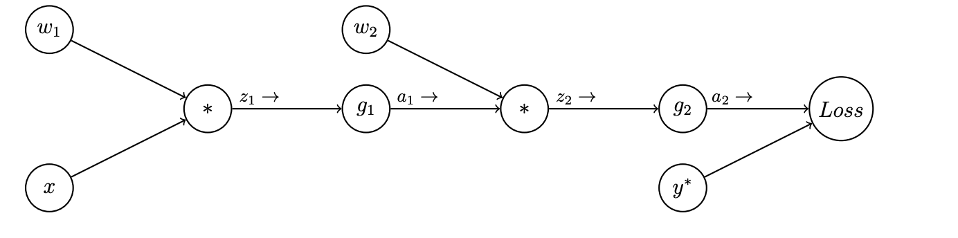
Consider the following computation graph for a simple neural network for binary classification. Here \(x\) is a single real-valued input feature with an associated class \(y^*\) (\(0\) or \(1\)). There are two weight parameters \(w_1\) and \(w_2\), and non-linearity functions \(g_1\) and \(g_2\). The network outputs \(a_2\) between 0 and 1, representing the probability of class 1. A loss function \(Loss\) is used to compare \(a_2\) with \(y^*\).

---

39.2.1 (a)

Perform the forward pass on this network, writing the output values for each node \(z_1, a_1, z_2, \text{and} \; a_2\) in terms of the node’s input values:

Answer

\[\begin{aligned} z_1 &= x * w_1 \\ a_1 &= g_1(z_1) \\ z_2 &= a_1 * w_2 \\ a_2 &= g_2(z_2) \end{aligned}\]

---

39.2.2 (b)

Compute the loss \(Loss(a_2, y^*)\) in terms of \(x\), \(w_i\), and \(g_i\):

Answer

Recursively substituting the values computed above, we have:

\[ Loss(a_2, y^*) = Loss\big(g_2(w_2 * g_1(w_1 * x)), y^*\big) \]

---

39.2.3 (c)

Now we will work through parts of the backward pass, incrementally. Use the chain rule to derive \(\frac{\partial Loss}{\partial w_2}\). Write your expression as a product of partial derivatives at each node: i.e. the partial derivative of the node’s output with respect to its inputs. (Hint: the series of expressions you wrote in part 1 will be helpful; you may use any of those variables.)

Answer

\[ \frac{\partial Loss}{\partial w_2} = \frac{\partial Loss}{\partial a_2} \frac{\partial a_2}{\partial z_2} \frac{\partial z_2}{\partial w_2} \]

---

39.2.4 (d)

Suppose the loss function is quadratic, \(Loss(a_2, y^*) = \frac{1}{2}(a_2-y^*)^2\), and \(a_1\) and \(a_2\) are both sigmoid functions \(g(z) = \frac{1}{1+e^{-z}}\) (note: it’s typically better to use a different type of loss, cross-entropy, for classification problems, but we’ll use this to make the math easier).

Using the chain rule from Part 3, and the fact that \(\frac{\partial g(z)}{\partial z} = g(z)(1-g(z))\) for the sigmoid function, write \(\frac{\partial Loss}{\partial w_2}\) in terms of the values from the forward pass, \(y^*\), \(a_1\), and \(a_2\).

Answer

First we’ll compute the partial derivatives at each node: \[\begin{aligned} \frac{\partial Loss}{\partial a_2} &= (a_2 - y^*) \\ \frac{\partial a_2}{\partial z_2} &= a_2(1 - a_2) \\ \frac{\partial z_2}{\partial w_2} &= a_1 \\ \end{aligned}\]

Now we can plug into the chain rule from part 3: \[ \frac{\partial Loss}{\partial w_2} = \frac{\partial Loss}{\partial a_2}\frac{\partial a_2}{\partial z_2}\frac{\partial a_2}{\partial w_2}\] \[ = (a_2 - y^*) * a_2(1 - a_2) * a_1 \]

---

39.2.5 (e)

Now use the chain rule to derive \(\frac{\partial Loss}{\partial w_1}\) as a product of partial derivatives at each node used in the chain.

Answer

\[ \frac{\partial Loss}{\partial w_1} = \frac{\partial Loss}{\partial a_2}\frac{\partial a_2}{\partial z_2}\frac{\partial z_2}{\partial a_1}\frac{\partial a_1}{\partial z_1}\frac{\partial z_1}{\partial w_1} \]

---

39.2.6 (e)

Finally, write \(\frac{\partial Loss}{\partial w_1}\) in terms of \(x, y^*, w_i, a_i, z_i\):

Answer

The partial derivatives at each node (in addition to the ones we computed in Part 4) are

\[ \begin{aligned} \frac{\partial z_2}{\partial a_1} &= w_2 \\ \frac{\partial a_1}{\partial z_1} &= \frac{\partial g_1(z_1)}{\partial z_1} = g_1(z_1)(1-g_1(z_1)) = a_1(1-a_1) \\ \frac{\partial z_1}{\partial a_1} &= x \end{aligned} \]

Plugging into the chain rule from Part 5 gives: \[ \begin{aligned} \frac{\partial Loss}{\partial w_1} &= \frac{\partial Loss}{\partial a_2}\frac{\partial a_2}{\partial z_2}\frac{\partial z_2}{\partial a_1}\frac{\partial a_1}{\partial z_1}\frac{\partial z_1}{\partial w_1} \\ &= (a_2-y^*) * a_2(1-a_2) * w_2 * a_1(1-a_1) * x \end{aligned} \]

---

39.2.7 (f)

What is the gradient descent update for \(w_1\) with step-size \(\alpha\) in terms of the values computed above?

Answer

\[ w_1 \leftarrow w_1 - \alpha * (a_2 - y^*) * a_2 (1 - a_2) * w_2 * a_1 (1 - a_1) * x \]