38 Discussion 11: Logistic Regression (From Summer 2025)
38.1 Logistic Regression
Suppose we are given the following dataset, with two features (\(\Bbb{X}_{:, 0}\) and \(\Bbb{X}_{:, 1}\)) and one binary response variable (\(y\)).
Here, \(\vec{x}^T\) corresponds to a single row of our data matrix, not including the \(y\) column. Thus, we can write \(\vec{x}_1^T\) as \(\vec{x}_1^T = \left[2 \quad 2\right]\). Note that there is no intercept term!
Suppose you run a Logistic Regression model to determine the probability that \(Y=1\) given \(\vec{x}\). We denote probability as \(P_{\hat{\theta}}\) as opposed to just \(P\) to show that \(\hat{\theta}\) is a learned parameter like it is in OLS, where we denote our function as \(f_{\theta}(x)\).
\[P_{\hat{\theta}}(Y=1|\vec{x}) = \sigma(\vec{x}^T \theta) = \frac{1}{1 + \exp(- \vec{x}^T \theta)}\]
Your algorithm learns that the optimal \(\hat\theta\) value is \(\hat\theta = \left[-\frac{1}{2} \quad-\frac{1}{2}\right]^T\).
38.1.1 (a)
\(\sigma(z)\) is called a “sigmoid” function, defined as
\[
\sigma(z) = \frac{1}{1 + \exp(-z)}
\]
for some arbitrary real number \(z\). What is the range of possible values for \(\sigma(\cdot)\)?
Answer
The range of the sigmoid function is \(0 < \sigma(z) < 1\). The function approaches 0 as \(z \to -\infty\) and approaches 1 as \(z \to +\infty\), but it never actually reaches either value. This is because the exponential function \(\exp(-z)\) grows very large for large negative \(z\), pushing the denominator to infinity (making \(\sigma(z)\) approach 0), and becomes very small for large positive \(z\), pushing the denominator toward 1 (making \(\sigma(z)\) approach 1).38.1.2 (b)
Calculate \(P_{\hat{\theta}}(Y=1|\vec{x}^T=\left[1 \quad 0\right])\).
Answer
\[ \begin{align*} P_{\hat{\theta}}(Y=1|\vec{x}^T=\left[1 \quad 0\right]) &= \sigma\left(\begin{bmatrix}1 & 0\end{bmatrix} \begin{bmatrix}-\frac{1}{2} \\ -\frac{1}{2}\end{bmatrix}\right) \\ &= \sigma\left(1 \cdot -\frac{1}{2} + 0 \cdot -\frac{1}{2}\right) \\ &= \sigma\left(-\frac{1}{2}\right) \\ &= \dfrac{1}{1 + \exp(\frac{1}{2})} \\ &\approx 0.38 \end{align*} \]38.1.3 (c)
Using a threshold of \(T=0.5\), what would our algorithm classify \(y\) as given the results of part b?
Answer
Our \(p\) of 0.38 is smaller than the threshold of 0.5, so our algorithm would classify y as class 0.38.1.4 (d)
The empirical risk using cross-entropy loss is given by the following expression. Remember, whenever you see \(\log\) in this course, you must assume the natural logarithm (base-\(e\)) unless explicitly told otherwise. \[ \begin{align*} R(\theta) &= -\dfrac{1}{n} \sum_{i=1}^{n} \big( y_i \log P_{\theta}(Y=1|\vec{x_i}) + (1-y_i) \log P_{\theta}(Y=0|\vec{x_i}) \big) \end{align*} \] Suppose we run a different algorithm and obtain \(\hat\theta_{new} = \left[0 \quad 0\right]^T\). Calculate the empirical risk for \(\hat\theta_{new}\) on our dataset.
Answer
\[ \begin{align*} R(\hat\theta_{new}) &= -\dfrac{1}{2} \sum_{i=1}^{2} \big( y_i \log P_{\hat{\theta_{new}}}(Y=1|\vec{x_i}) + (1-y_i) \log P_{\hat{\theta_{new}}}(Y=0|\vec{x_i}) )\\ &= -\frac{1}{2} [(0 \log P_{\hat{\theta_{new}}}(Y=1|\vec{x_1}) + 1 \log P_{\hat{\theta_{new}}}(Y=0|\vec{x_1})) + \\ & (1 \log P_{\hat{\theta_{new}}}(Y=1|\vec{x_2}) + 0 \log P_{\hat{\theta_{new}}}(Y=0|\vec{x_2}))] \\ &= -\frac{1}{2} (\log P_{\hat{\theta_{new}}}(Y=0|\vec{x_1}) + \log P_{\hat{\theta_{new}}}(Y=1|\vec{x_2})) \\ &= -\frac{1}{2} (\log (1 - \sigma(0)) + \log \sigma(0)) \\ &= -\log(0.5) = \log 2 \approx 0.693 \\ \end{align*} \]38.1.5 (e) (Extra)
Consider using a linear regression model such that \(\hat{\mathbb{Y}} = \mathbb{X}\hat{\theta}\). What is the MSE of the optimal linear regression model given the dataset we used above?
Answer
The loss is zero - the design matrix is full rank and square, so we can invert it to find a perfect mapping from the explanatory variable to the response variable!38.2 More Linear Regression
Suppose we have two different Logistic Regression models, A and B, and we run gradient descent for 1000 steps to obtain the model parameters \(\hat\theta_A = \left[-\frac{1}{2} \quad-\frac{1}{2}\right]^T\) and \(\hat\theta_B = \left[0 \quad0\right]^T\). How do they compare?
The dataset is reproduced below for your convenience.
| \(\mathbb{X}_{:, 0}\) | \(\mathbb{X}_{:, 1}\) | \(y\) |
|---|---|---|
| 2 | 2 | 0 |
| 1 | -1 | 1 |
38.2.1 (a)
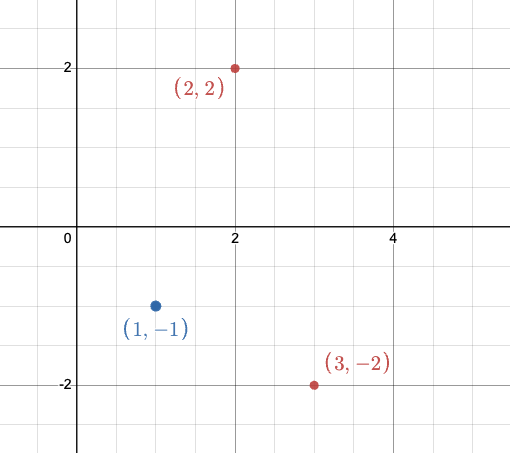
Is our dataset linearly separable? If so, write the equation of a hyperplane that separates the two classes. Otherwise, briefly explain why not (Hint: draw the two data points).
Answer
Yes, the line \(\Bbb{X}_{:, 1} = 0\) separates the data in feature space.

Since this dataset has only 2 points in 2D, it’s a great opportunity to draw it out on a coordinate plane.
- Plot the two points and label them clearly.
- Notice that there are many possible separating lines (or hyperplanes) that can divide these points into different classes.
- This is a good chance to see how in higher dimensions, multiple valid separating boundaries can still exist.
38.2.2 (b)
If we let gradient descent keep running indefinitely for our two models, will either of them converge given the design matrix above? Why? If not, how can we remedy this?
Answer
No.
Our dataset is linearly separable, so the optimal cross-entropy loss is 0. However, a cross-entropy loss of 0 can never be achieved. Remember that \(\sigma(z)\) never outputs precisely 0 or 1, but it can get arbitrarily close. Hence, no single value of \(\theta\) will ever “minimize” cross-entropy loss (ie. let \(\sigma(x^T \theta) = 0\)), but gradient descent can bring the cross-entropy loss closer and closer to 0 as \(\theta\) goes to \(\pm \infty\).
To avoid our absolute values of the weights diverging to \(\infty\), we can regularize our cross-entropy loss.
Note: In the real world, since computers have finite precision (decimals can only go so far) it will eventually converge. But without this limitation, in the ideal world gradient descent will never converge.38.2.3 (c)
Assume we add the data point \([3, -2]\) to the design matrix such that our resulting design matrix is as follows.
| \(\mathbb{X}_{:, 0}\) | \(\mathbb{X}_{:, 1}\) | \(y\) |
|---|---|---|
| 2 | 2 | 0 |
| 1 | -1 | 1 |
| 3 | -2 | 0 |
Is it possible to achieve perfect accuracy using a logistic regression model?
Answer
The data is still linearly separable, so we can train a logistic regression model to achieve perfect accuracy!
38.2.4 (d) (Extra)
Secondly, what would happen if we were to train a linear regression model on the above data? Interpret the meaning of the predictions and MSE. (Assume there is an intercept term)
Answer
We need a full rank matrix to have a unique solution with some MSE. However, the MSE that is returned, the mean squared error in the training set, is how far off our \(\hat{y}\) is from the NUMBERS 1 or 0. We can not directly interpret this as a probability since our model can output \(\hat{y}\) values above 1 and below 0.38.3 Deriving Logistic Regression (Extra)
This question is designed to help you see how the equation for logistic regression is derived by starting from the linear regression equation and transforming it step-by-step into the logistic regression equation.
- The process here goes in the opposite order from lecture, where we moved from the logistic regression equation back to the linear regression equation.
- Before starting, make sure you’re clear on the difference between square brackets
[]and parentheses(), since both appear in the equations.
Goal: By the end, you should understand the reasoning behind the (sometimes unintuitive) logistic regression formula and how it relates to linear regression.
In this question, we’ll walk through a transformation from the Linear Regression equation to the Logistic Regression equation.
The goal of Linear Regression is to predict \(y\) given an input \(y\), and this is accomplished by learning the parameter \(\theta\). While this model can be useful when predicting things like house prices in Project A, it does less well when predicting binary variables of 0 or 1.
38.3.1 (a)
How can we modify our Linear Regression equation, \(y = x^T \theta\), to fit this new type of problem? Instead of predicting the value of \(y\), which can only be 0 or 1, let’s predict the probability \(p\) that \(y=1\). Under this model, what’s the probability that \(y=0\)? What is the range of values that \(p\) could take?
Answer
Since \(P[y=1]\), and Y can only take on 2 values, \(P[y=0]\) must be \(1-p\).
\(0 \le p \le 1\) because \(p\) is a probability.38.3.2 (b)
Our goal is to modify our original function, \(x^T \theta\), so that it’s range of values is [0, 1] instead of (\(-\infty\), \(+\infty\)). To do this, we’ll perform a series of transformations on \(x^T \theta\) starting with “odds”. Odds is the ratio of the probability of \(y\) being Class 1 to the probability of \(y\) being Class 0. \[odds = \frac{P(y=1 | x)}{P(y=0 | x)} = \frac{p}{1-p} \]
What is the range of \(odds\)?
Answer
The range of \(p\) is constrained from 0 to 1. \[\lim_{p \to 0} = 0\] \[\lim_{p \to 1} = + \infty\]
Remember that the range of the odds function is determined by the range of the probability \(p\).
- Since \(0 < p < 1\) for probabilities, the odds \(\frac{p}{1-p}\) can only take on positive values.
- As \(p\) approaches 0, the odds approach 0.
- As \(p\) approaches 1, the odds grow without bound.
Key takeaway: The possible values of the odds are directly limited by the fact that probabilities are always between 0 and 1.
38.3.3 (c)
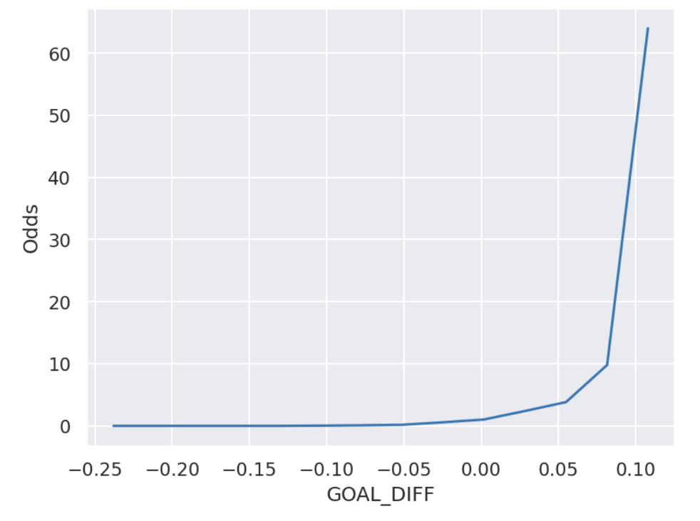
Notice how the \(odds\) plot bulges to the bottom right quadrant (recall the Tukey-Mosteller diagram). Thus, the final transformation we’ll perform is a log. \[log(odds) = log(\frac{p}{1-p})\] What is the range of \(log(odds)\)? Does it match the range of our Linear Regression model?
Answer
38.3.4 (c)
Putting this all together, we get \[ log(\frac{p}{1-p}) = x^T \theta\] Rearranging the terms, we can solve for p: \[p = \frac{1}{1 + e^{-x^T \theta}} = \sigma(x^T \theta)\] and obtain our logistic function \(\sigma()\). What is the range of values that \(\sigma()\) could take?
Answer
38.4 Extra Linear Regression (Extra)
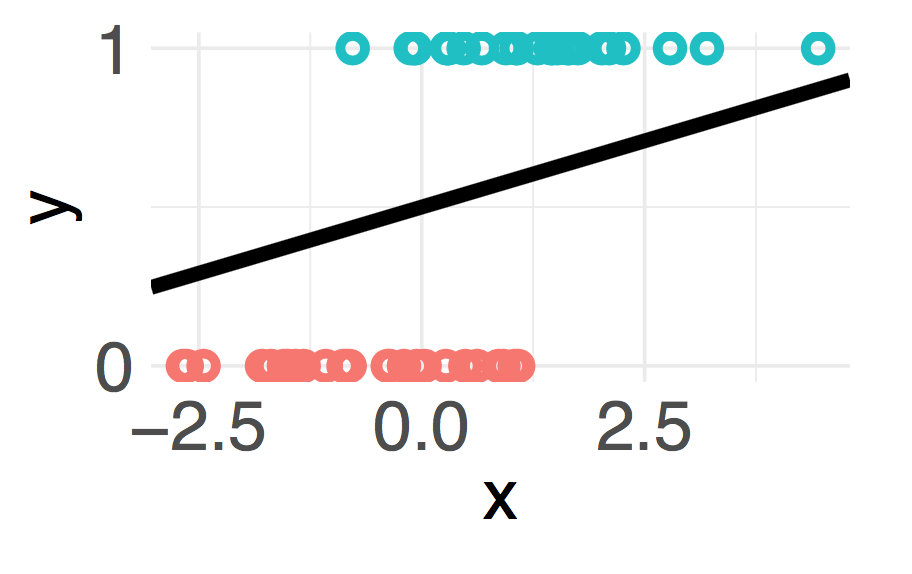
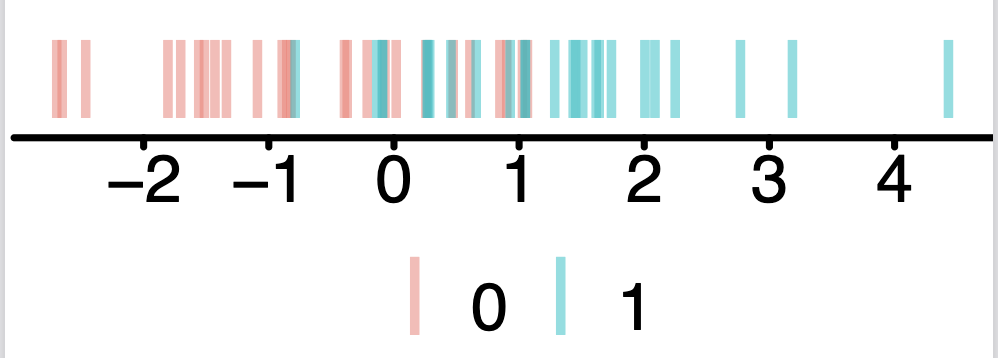
Your friend working on a different problem obtains a different dataset with a single feature \(x\). Your friend argues that the data are linearly separable by drawing the line on the following data plot.
38.4.1 (a)
Is your friend correct? Explain your reasoning. Note: This question refers to a binary classification problem with a single feature.
Answer
The scatter plot of \(x\) against \(y\) isn’t the graph you should look at. The more salient plot would be the 1D representation of the features colored by class labels. Linear separability is defined in the feature space.
38.4.2 (b)
Suppose you use gradient descent for a fixed number of iterations to train a logistic regression model on two design matrices \(\Bbb{X}_a\) and \(\Bbb{X}_b\). After training, the training accuracy for \(\Bbb{X}_a\) is 100%, and the training accuracy for \(\Bbb{X}_b\) is 98%. What can you say about whether the data is linearly separable for the two design matrices?