33 Discussion 06: Modeling & OLS (From Summer 2025)
33.1 Driving with a Constant Model
Lillian is trying to use modeling to drive her car autonomously. To do this, she collects a lot of data from driving around her neighborhood and stores it in drive. She wants your help to design a model that can drive on her behalf in the future using the outputs of the models you design. First, she wants to tackle two aspects of this autonomous car modeling framework: going forward and turning.
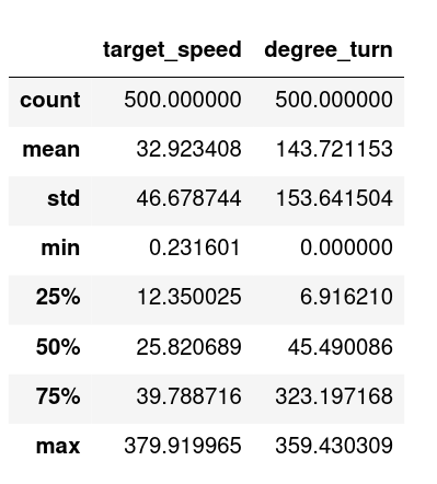
Some statistics from the collected dataset are shown below using drive.describe(), which returns the mean, standard deviation, quartiles, minimum, and maximum for the two columns in the dataset: target_speed and degree_turn.
33.1.1 (a)
Suppose the first part of the model predicts the target speed of the car. Using constant models trained on the speeds of the collected data shown above with \(L_1\) and \(L_2\) loss functions, which of the following is true?
Answer
When we train the model with \(L_1\) loss, the optimal value \(\hat{\theta}\) is the median of all the target speeds. From the summary statistics, the median value is indicated by the 50% percentile value, namely, \(\approx25.82\).
When training with \(L_2\) loss, \(\hat{\theta}\) is the mean of all the target speeds, which happens to be \(\approx32.92\). Since the mean is larger than the median, the constant model trained with \(L_2\) loss will always result in a higher speed than when trained with \(L_1\) loss.33.1.2 (b)
Finding that the model trained with the \(L_2\) loss drives too slowly, Lillian changes the loss function for the constant model where the loss is penalized more if the true speed is higher. That way, in order to minimize loss, the model would have to output predictions closer to the true value, particularly as speeds get faster, the end result being a higher constant speed. Lillian writes this as \(L(y, \hat{y}) = y(y - \hat{y})^2\).
Find the optimal \(\hat{\theta_0}\) for the constant model using the new empirical risk function \(R(\theta_0)\) below:
\[ R(\theta_0) = \frac{1}{n} \sum_i y_i (y_i - \theta_0)^2 \]
Answer
Take the derivative:
\[ \frac{dR}{d\theta_0} = \frac{1}{n} \sum_i \frac{d}{d\theta_0} y_i (y_i - \theta_0)^2 = \frac{1}{n} \sum_i -2y_i (y_i - \theta_0) = -\frac{2}{n} \sum_i y_i^2 - y_i \theta_0 \]
Set the derivative to 0:
\[ -\frac{2}{n} \sum_i y_i^2 - y_i\theta_0 = 0 \]
\[ \theta_0 \sum_i y_i = \sum_i y_i^2 \]
\[ \theta_0 = \frac{\sum_i y_i^2}{\sum_i y_i} \]
Note that the empirical risk function is convex, which you can show by computing the second derivative of \(R(\theta_0)\) and noting that it is positive for all values of \(\theta_0\).
\[\frac{d^2R}{d\theta_0^2} = \frac{2}{n} \sum_i y_i > 0\] since \(y_i\) represents speed, also validated by the fact that the minimum value is positive.
Therefore, any critical point must be the global minimum and so the optimal value we found minimizes empirical risk.33.1.3 (c) (Extra)
To upgrade her model to be able to use a feature \(x\), Lillian uses a simple linear regression model without an intercept term; that is, the model is given by \(y = \theta x\). Using the standard \(L_2\) loss, what is the optimal \(\theta\) that minimizes the following empirical risk?
\[ R(\theta) = \frac{1}{n} \sum_i (y_i - \theta x_{i})^2 \]
Answer
\[ \begin{align*} \frac{d}{d\theta} R(\theta) &= \frac{1}{n}\sum_{i=1}^{n} \frac{d}{d\theta}(y_{i} - \theta x_{i})^{2} \\ &= -\frac{2}{n}\sum_{i=1}^{n} x_{i}(y_{i} - \theta x_{i}) \end{align*} \]
Setting to \(0\) and solving for \(\theta\):
\[ \begin{align*} -\frac{2}{n}\sum_{i=1}^{n} x_{i}(y_{i} - \hat{\theta} x_{i}) &= 0 \\ \sum_{i=1}^{n} x_{i}(y_{i} - \hat{\theta} x_{i}) &= 0 \\ \sum_{i=1}^{n} x_{i}y_{i} - \hat{\theta} \sum_{i=1}^{n} x_{i}^{2} &= 0 \\ \hat{\theta} &= \frac{\sum_{i=1}^{n}x_{i}y_{i}}{\sum_{i=1}^{n}x_{i}^{2}} \end{align*} \]
33.1.4 (d)
Lillian’s friend, Yash, also begins working on a model that predicts the degree of turning at a particular time between 0 and 359 degrees using the data in the degree_turn column. Explain why a constant model is likely inappropriate in this use case.
Extra: If you’ve studied some physics, you may recognize the behavior of our constant model!
Answer
Any constant model will essentially be always turning at an angle and will be unable to turn either direction or go straight (i.e. it’ll essentially go in a circle forever).33.1.5 (e)
Suppose we finally expand our modeling framework to use simple linear regression (i.e. \(f_\theta(x) = \theta_{w,0} + \theta_{w,1}x\)). For our first simple linear regression model, we predict the turn angle (\(y\)) using target speed (\(x\)). Our optimal parameters are: \(\hat{\theta}_{w,1} = 0.019\) and \(\hat{\theta}_{w,0} = 143.1\).
However, we realize that we actually want a model that predicts target speed (our new \(y\)) using turn angle, our new \(x\) (instead of the other way around)! What are our new optimal parameters for this new model?
Answer
To predict target speed (new \(y\)) from turn angle (new \(x\)) (what we finally want), we need to compute \(\hat{\theta}_1 = \frac{r\sigma_{\text{speed}}}{\sigma_{\text{turn}}}\).
When we predicted the turn angle from target speed (our first SLR model), we computed \(\hat{\theta}_{w,1} = \frac{r \sigma_{\text{turn}}}{\sigma_{\text{speed}}}\). To go from \(\hat{\theta}_{w,1}\) to \(\hat{\theta}_1\), we multiply by \(\frac{\sigma^2_{\text{speed}}}{\sigma^2_{\text{turn}}}\).
That is, \(\hat{\theta}_1 = \frac{r\sigma_{\text{speed}}}{\sigma_{\text{turn}}} = (\frac{r \sigma_{\text{turn}}}{\sigma_{\text{speed}}}) \frac{\sigma^2_{\text{speed}}}{\sigma^2_{\text{turn}}} = \hat{\theta}_{w,1} \frac{\sigma^2_{\text{speed}}}{\sigma^2_{\text{turn}}} = 0.019 \cdot \frac{46.678744^2}{153.641504^2} = 0.00175\).
Then, \(\hat{\theta}_0 = \bar{y} - \hat{\theta}_1 \bar{x} = 32.92 - 0.00175 \cdot 143.72 = 32.67\).
\(\bar{y}\) and \(\bar{x}\) refer to the means of target speed (our new \(y\)) and turn angle (our new \(x\)) respectively.
Note: we can’t use the inverse function \(f_\theta^{-1}(x)\) since minimizing the sum of squared verticals is not the inverse problem of minimizing the sum of squared horizontal residuals.
Have you ever wondered why we can’t just flip the regression line and use the inverse function \(f_\theta^{-1}(x)\)? The reason is that regression is directional.
In simple linear regression (SLR), we minimize the sum of squared vertical distances from the data points to the line. This is different from minimizing the horizontal distances. So switching \(x\) and \(y\) does not give you the inverse regression line.
For example:
- When predicting \(y\) from \(x\), the slope is
\[ m_1 = \frac{r \sigma_y}{\sigma_x} \]
- When predicting \(x\) from \(y\), the slope is
\[ m_2 = \frac{r \sigma_x}{\sigma_y} \]
These slopes are not inverses of each other.
The figures below help visualize this:

Here you can see the difference in regression direction. The first figure shows how the line changes when swapping \(x\) and \(y\), and the second figure shows vertical vs. horizontal residuals:
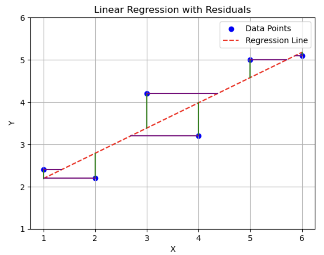
Key takeaway: Minimizing squared residuals in different directions gives different slopes. Always choose the regression direction based on what you want to predict.
33.2 Geometry of Least Squares
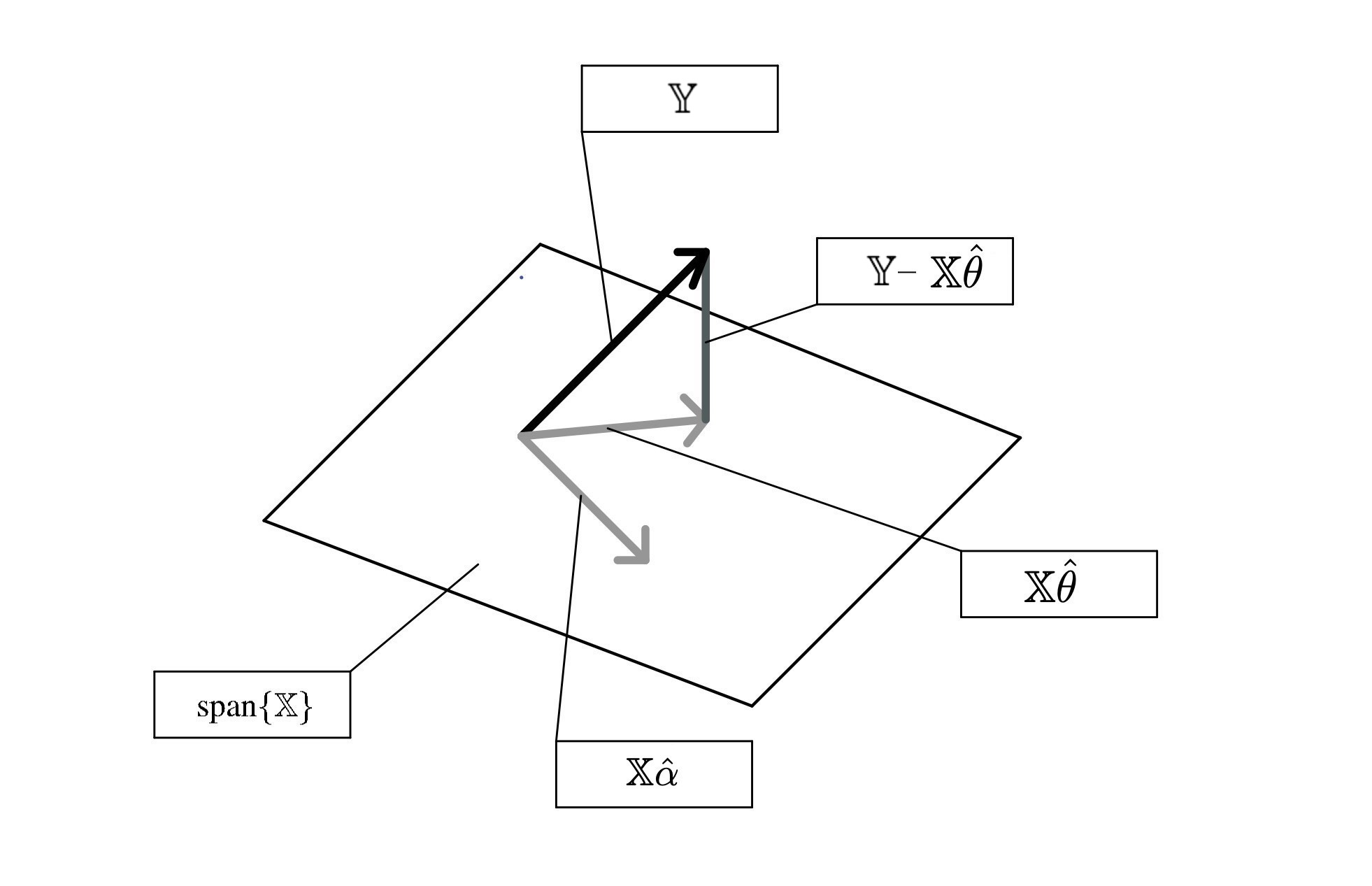
Suppose we have a dataset represented with the design matrix \(\text{span}(\mathbb{X})\) and response vector \(\mathbb{Y}\). We use linear regression to solve for this and obtain optimal weights as \(\hat{\theta}\). Label the following terms on the geometric interpretation of ordinary least squares:
- \(\mathbb{X}\) (i.e., \(\text{span}(\mathbb{X})\))
- The response vector \(\mathbb{Y}\)
- The residual vector \(\mathbb{Y} - \mathbb{X}\hat{\theta}\)
- The prediction vector \(\mathbb{X}\hat{\theta}\) (using optimal parameters)
- A prediction vector \(\mathbb{X}{\alpha}\) (using an arbitrary vector \(\alpha\))
![]()
Answer
33.3 More Geometry of Least Squares
Using the geometry of least squares, let’s answer a few questions about Ordinary Least Squares (OLS)!
33.3.1 (a)
Which of the following are true about the optimal solution \(\hat{\theta}\) to OLS? Recall that the least squares estimate \(\hat{\theta}\) solves the normal equation \((\Bbb{X}^T\Bbb{X})\theta = \Bbb{X}^T\Bbb{Y}\).
\[\hat{\theta} = (\Bbb{X}^T\Bbb{X})^{-1}\Bbb{X}^T\Bbb{Y}\]
Answer
We can derive solutions to both simple linear regression and constant model with an \(L_2\) loss since they can be represented in the form \(y = x^T\theta\) in some way. Specifically, one of the two entries of \(x\) would be 1 for SLR (and the other would be the explanatory variable). The only entry for the constant model would be 1.
We cannot derive solutions for anything with the \(L_1\) loss since the normal equation optimizes for MSE.
Since option E is linear with respect to \(\theta\), we can use the normal equation. A good rule of thumb to determine if an equation is linear to \(\theta\) is checking if an expression can separate into a matrix product of two terms:
In simple linear regression, we can write the prediction vector as:
\[ \hat{y} = \begin{bmatrix} x & \sin(x^2) \end{bmatrix} \begin{bmatrix} \theta_1 \\ \theta_2 \end{bmatrix} \]
This is linear in the parameters \(\theta_1\) and \(\theta_2\), so we can use the normal equations to solve for the optimal parameters.
Conversely, option F is not linear in \(\theta\), which means the normal equations cannot be applied in that case.33.3.2 (b)
Which of the following conditions are required for the least squares estimate in the previous subpart?
Answer
\(\Bbb{X}\) must be full column rank in order for the normal equation to have a unique solution. If \(\Bbb{X}\) is not full column rank, then \(\Bbb{X}^T\Bbb{X}\) is not invertible, and the least squares estimate will not be unique. Note that neither \(\Bbb{X}\) nor \(\Bbb{X}^T\) needs to be invertible. Also, \(\Bbb{Y}\) is a vector, so the idea of it being “full column rank” doesn’t apply—it always has rank at most 1. Its specific values (e.g., being the zero vector) do not affect whether the least squares estimate exists or is unique.
You don’t need to know the full math proof showing why \(X\) being full column rank implies that \(X^TX\) is invertible — this was just mentioned in lecture.
If you’re curious, some bonus material covering this is included at the end of Lecture 12.
33.3.3 (c)
What is always true about the residuals in the least squares regression? Select all that apply.
Answer
C: C is wrong because the mean squared error is the mean of the sum of the squares of the residuals.\
D: A counter-example is: \(\mathbb{X} = \begin{bmatrix} 2 & 3 \\ 1 & 5 \\ 2 & 4 \end{bmatrix}, \mathbb{Y} = \begin{bmatrix} 1 \\ 3 \\ 2 \end{bmatrix}\). After solving the least squares problem, the sum of the residuals is \(-0.0247\), which is not equal to zero. However, note that this statement is, in general, true if every feature contains the same constant intercept term. \
E: is wrong since A and B are correct.33.3.4 (d)
Which of the following are true about the predictions made by OLS? Select all that apply.
Answer
A is correct because they are linear projections onto the column space. This fact also makes C correct, E incorrect, and D incorrect.
B is correct based on the definition of OLS.33.3.5 (e) (Extra)
We fit a simple linear regression to our data \((x_i, y_i)\) for \(i \in \{1, 2, \dots, n\}\), where \(n\) is the number of samples, \(x_i\) is the independent variable, and \(y_i\) is the dependent variable. Our regression line is of the form \(\hat{y} = \hat{\theta_0} + \hat{\theta_1}x\). Suppose we plot the relationship between the residuals of the model and the \(\hat{y}_i\)’s and find that there is a curve. What does this tell us about our model?
Answer
33.3.6 (f)
Which of the following is true of the mystery quantity \(\vec{v} = (I - \Bbb{X}(\Bbb{X}^T\Bbb{X})^{-1}\Bbb{X}^T) \Bbb{Y}\)?
Answer
A is incorrect because any linear model does not create the residual vector \(v\); only the optimal linear model does.
D is incorrect because the vector \(v\) is of size \(n\) since there are \(n\) data points.
The rest are correct by properties of orthogonality as given by the geometry of least squares.
We won’t show the proof that the average of residuals is 0 — that’s something you’ll work on in the homework!
33.3.7 (g)
Derive the least squares estimate \(\hat{\theta}\) by leveraging the geometry of least squares.
Note: While this isn’t a “proof” or “derivation” class (and you certainly will not be asked to derive anything of this sort on an exam), we believe that understanding the geometry of least squares enough to derive the least squares estimate shows great understanding of all the linear regression concepts we want you to know! Additionally, it provides great practice with tricky linear algebra concepts such as rank, span, orthogonality, etc.
Answer
We know that the best estimate of \(\mathbb{Y}\) is such that everything that we cannot represent or get to (i.e. the residuals) is orthogonal to what we can represent or get to (i.e. the span). Mathematically, we then know that every vector in \(\mathbb{X}\) and \(\mathbb{Y} - \hat{\mathbb{Y}}\) are orthogonal.
We know that when two vectors \(u, v\) are orthogonal, \(u^Tv = 0\). Using this fact, we can then know that for any (column) vector \(x_i\) in \(\mathbb{X}\), that \(x_i^T(\mathbb{Y} - \hat{\mathbb{Y}}) = 0\).
When we write this out for all our column vectors, we know that this entire quantity is just the zero vector! (note that \(x_1\) could be a vector of all 1’s and could thus be \(\mathbb{1}^T (\mathbb{Y} - \hat{\mathbb{Y}})\))
\[\begin{bmatrix} x_1^T(\mathbb{Y} - \hat{\mathbb{Y}}) \\ x_2^T(\mathbb{Y} - \hat{\mathbb{Y}})\\ ... \\ x_p^T(\mathbb{Y} - \hat{\mathbb{Y}}) \end{bmatrix} = \mathbb{X}^T(\mathbb{Y} - \hat{\mathbb{Y}}) = 0\]
From here, all that is left is algebra! Recall from our linear model that \(\hat{\mathbb{Y}} = \mathbb{X} \hat{\theta}\).
\[ \mathbb{X}^T\mathbb{Y} = \mathbb{X}^T\hat{\mathbb{Y}} = \mathbb{X}^T\mathbb{X} \hat{\theta} \]
We know for a fact that \(\mathbb{X}^T\mathbb{X}\) has to be square, but it may or may not be invertible depending on one particular condition (take a look at Question 2 part b). In this case, it is:
\[ \hat{\theta} = ( \mathbb{X}^T\mathbb{X})^{-1} \mathbb{X}^T\mathbb{Y} \]33.4 Modeling using Multiple Regression (Extra)
Ishani wants to model exam grades for DS100 students. She collects various information about student habits, such as how many hours they studied, how many hours they slept before the exam, and how many lectures they attended and observes how well they did on the exam. Suppose she collected such information on \(n\) students, and wishes to use a multiple-regression model to predict exam grades.
33.4.1 (a)
Using the data from the \(n\) individuals, she constructs a design matrix \(\mathbb{X}\) and uses the OLS formula to obtain the estimated parameter vector:
\[ \hat{\theta} = \begin{bmatrix} 3 \\ 2 \\ 1 \end{bmatrix} \]
The design matrix \(\mathbb{X}\) was constructed so that:
- The first column represents how many hours each student studied.
- The second column represents how many hours each student slept before the exam.
- The third column represents how many lectures each student attended.
With this in mind, interpret each entry of \(\hat{\theta}\) in context. For example:
- \(\hat{\theta}_1 = 3\) means that, holding sleep and lectures constant, each additional hour of study is associated with an expected increase of 3 points on the exam.
- \(\hat{\theta}_2 = 2\) means that, holding study hours and lectures constant, each additional hour of sleep is associated with an expected increase of 2 points.
- \(\hat{\theta}_3 = 1\) means that, holding study hours and sleep constant, attending one more lecture is associated with an expected increase of 1 point.
Answer
Each regression coefficient (component of vector) represents the amount we expect an individual’s exam score to go up when increasing the corresponding variable by one unit and holding all other variables fixed. For instance, for the first component, when holding ‘hours of sleep’ and ‘lectures attended’ constant, an individual’s score is expected go up by 3 per extra hour spent studying. The other components can be interpreted similarly.
It can help to write out the fitted models and explicitly see what happens when you increase one covariate by 1 while holding all other covariates fixed. This makes it easier to interpret each parameter in context.
33.4.2 (b)
After fitting this model, we would like to predict the exam grades for two individuals using these variables. Suppose for Individual 1, they slept 10 hours, studied 15 hours, and attended 4 lectures. Suppose also for Individual 2, they slept 5 hours, studied 20 hours, and attended 10 lectures. Construct a matrix \(\mathbb{X}'\) such that, if you computed \(\mathbb{X}'\hat{\theta}\), you would obtain a vector of each individual’s predicted exam scores.
Answer
\[ \mathbb{X}' = \begin{bmatrix} 15 & 10 & 4 \\ 20 & 5 & 10 \end{bmatrix} \]33.4.3 (c)
Denote \(y'\) as a \(2 \times 1\) vector that represents the actual exam scores of the individuals Ishani is predicting on. Write out an expression that evaluates to give the Mean Squared Error (MSE) of our predictions using matrix notation.