20  Discussion 05: Transformation, Probability & Sampling (From Summer 2025)

Slides

20.1 Logarithmic Transformations

Ishani is a development economist interested in studying the relationship between literacy rates and gross national income in countries across the world. Originally, she plotted the data on a linear (absolute) scale, shown on the left. She noticed that the non-linear relationship between the variables with a lot of points clustered towards the larger values of literacy rate, so she consults the Tukey-Mosteller Bulge diagram and decides to do a \(\log_{10}\) transformation of the y-axis, shown on the right. The solid blue line is a “line of best fit” (we’ll formalize this later in the course).

Understanding the Purpose of Log Transformation

The goal here is to think about the meaning of the \(\log\) transformation, not just memorize “when to log-transform” data. The problem setup gives you a visual cue to guide your thinking.

For part (a), consider when the other descriptions might also be appropriate.

Remember: log-transforming data reduces the impact of large values by making them smaller, which can make patterns in the data easier to see.

---

20.1.1 (a)

Instead of using the \(\log_{10}\) transformation of the y-axis, what other transformations could Ishani have used to attempt to linearize the relationship between literacy rate (\(x\)) and gross national income per capita (\(y\)). Select all that apply.

• \(\log_{e}(y)\)
• \(10^y\)
• \(\sqrt{x}\)
• \(x^2\)
• \(y^2\)

Answer

• \(\log_{e}(y)\)
• \(x^2\)

The shape of the plot on the absolute scale suggests that a nonlinear transformation may help linearize the relationship. Possible transformations to consider include \(x^3\) and \(\sqrt{y}\). Note that the base of the logarithm is not generally specified—both base 10 and base \(e\) (or even other bases) can be effective in achieving linearity. The choice of base may depend on the degree and direction of skewness in the data.

---

20.1.2 (b)

Let \(C\) and \(k\) be some constant values and \(x\) and \(y\) represent literacy rate and gross national income per capita, respectively. Based on the plots, which of the following best describes the pattern seen in the data?

• \(y = C + kx\)
• \(y = C \times 10^{kx}\)
• \(y = C + k\log_{10}(x)\)
• \(y = Cx^k\)

Answer

• \(y = C \times 10^{kx}\)

\(y = kx + b\) is the basic format of the regression line. Since the graph on the right takes the log scale of the y-axis, we can write the equation as \(\log_{10}y = kx + b\) and manipulate it until we get \(y\) on it’s own: \[ \begin{align} \log_{10}(y) &= kx + b \\ 10^{\log_{10}(y)} &= 10^{kx + b} \\ y &= 10^{kx} \cdot 10^b \\ y &= 10^b \cdot 10^{kx} \end{align} \]

Hence, this equation format fits choice B, \(y = C \cdot 10^{kx}\), where \(C = 10^b\).

---

20.1.3 (c)

What parts of the plots could you use to make initial guesses on \(C\) and \(k\)?

Answer

• C: \(10^b\), where \(b\) is the y-intercept of the solid blue line in the transformed plot.
• k: the slope of the solid blue line in the transformed plot.

---

20.1.4 (d)

Ishani’s friend, Yash, points to the solid line on the transformed plot and says “since this line is going up and to the right, we can say that, in general, the higher the literacy rate, the greater the gross national income per capita”. Is this a reasonable interpretation of the plot?

Answer

Yes, the observation is equivalent to saying that the slope is positive, which means increases in \(x\) correspond to increases in \(y\). This does not mean higher literacy rates cause higher gross national incomes, just that they are positively correlated.

---

20.1.5 (e)

Suppose that instead of plotting positive quantities, our data contained some zero and negative values. How can we reasonably apply a logarithmic transform to this data?

Answer

Logs cannot take on zero or negative values, so we must shift our data into positive quantities before applying a logarithmic transform. To achieve this, we add the magnitude (or absolute value) of the most negative number in our data and then add a small positive number (e.g., 1). As a concrete example, suppose we had the dataset: \({-3, -2, 4}\). The most negative number is -3, so we add \(|-3| = 3\) to all numbers to obtain: \({0, 1, 7}\). This fixes the issue with negative values, but this dataset still contains the value 0. Hence, we add a small positive number such as 1, to get the numbers \({1, 2, 8}\) that we can finally apply the \(log\) operation to.

---

20.1.6 (f) (Extra)

They go on to say “since the slope of this line is less than 1, we see that, in general, mammals with greater mass tend to spend less energy per gram than their smaller counterparts”. Is this a reasonable interpretation of the plot?

Answer

Yes, a slope between 0 and 1 means that \(k\) is likely between 0 and 1. Looking at \(\frac{dy}{dx}\), we see that for these values of \(k\), as \(x\) grows, its effect on \(y\) diminishes. In this case, it means that gram-for-gram larger mammals spend less energy than their smaller counterparts.

20.2 Data Collection through Sampling

It’s time for the Data 100 midterm, and the professors want to estimate the difficulty of the exam. They decided to survey students on the exam’s difficulty with a 10-point scale and then use the mean of the student’s responses as the estimate.

---

20.2.1 (a)

What is the population the professors are interested in trying to understand?

• Students in Data 100
• Students enrolled in the Data 100 Ed
• Students who attend the Data 100 lectures
• Students who took the Data 100 midterm

Answer

• Students who took the Data 100 midterm

Some students enrolled in Data 100, on Ed, or who attend lectures may not have taken the midterm exam. We only want to survey students who actually took the exam, so (D) is the correct choice.

---

20.2.2 (b)

The professors consider a few different methods for collecting the survey data about the midterm. Which of the following methods is best? (Think through which considerations go into “best”)

• The professors add one Slido poll in the first lecture following the exam and only consider synchronous responses.
• The professors add a question to the homework assignments of a simple random sample of students.
• The professors choose a simple random sample of discussion sections, go to each selected section and ask each student during the section.
• The professors choose a simple random sample of discussion sections, go to each selected section and ask each student in the group as part of the final discussion question.

Answer

• The professors add a question to the homework assignments of a simple random sample of students.
  

1. It would be a fairly easy method. However, the quality of the data would be suspect. By sampling only from students who attend synchronously, the professors are restricting students who prefer not to attend live sessions. These can introduce selection bias in the sample.
2. This method of sampling works well for this scenario because the professors are sampling randomly from students across different backgrounds and schedules, which helps capture variation along many axes. They are also embedding the question in required homework, which reduces non-response bias, and students can respond privately, reducing social desirability bias.
3. This method is not ideal because discussion attendance is not mandatory this semester, which introduces selection bias—only students who choose to attend discussions will be included. As a result, the sample may not be representative of the entire class. Additionally, asking students during the section could increase social desirability bias, as students may feel pressure to respond in a certain way in front of peers or instructors.
4. The primary issue here is one of social pressure because students are being asked in groups, and this can bias the results of the survey. Additionally, discussion attendance isn’t mandatory this semester, and there’s bias from who chooses to attend.

Evaluating Sampling Methods

Each sampling method has its strengths and weaknesses, but choice B is generally the best option.

Think about the pros and cons of each method. For example, even choice B leaves out students who don’t look at or complete their homework.

Take some time to discuss the advantages and disadvantages of each option — there’s often no perfect method, but weighing trade-offs helps you choose the most appropriate one.

20.3 Simple Linear Regression

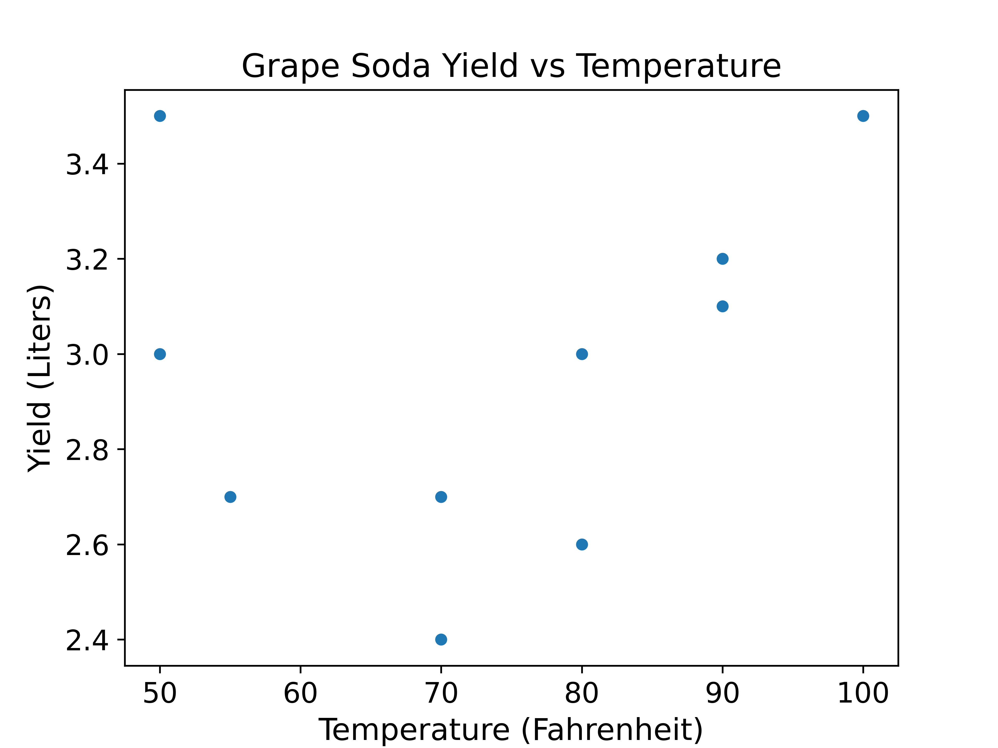
Lillian and Prabhleen were watching their favorite chemistry Youtuber NileRed experimenting with turning gloves into grape soda and wanted to try it themselves. The experiment was done at various temperatures and yielded various amounts of grape soda. Since this reaction is very costly, they were only able to do it 10 times. This data set of size \(n = 10\) (Yield data) contains measurements of yield from an experiment done at five different temperature levels. The variables are \(y\) = yield in liters and \(x\) = temperature in degrees Fahrenheit. Below is a scatter plot of our data.

\(\sigma_x\)	\(\sigma_y\)	\(r\)	\(\bar{x}\)	\(\bar{y}\)
\(15\)	\(0.3\)	\(0.50\)	\(75.00\)	\(3\)

20.3.1 (a)

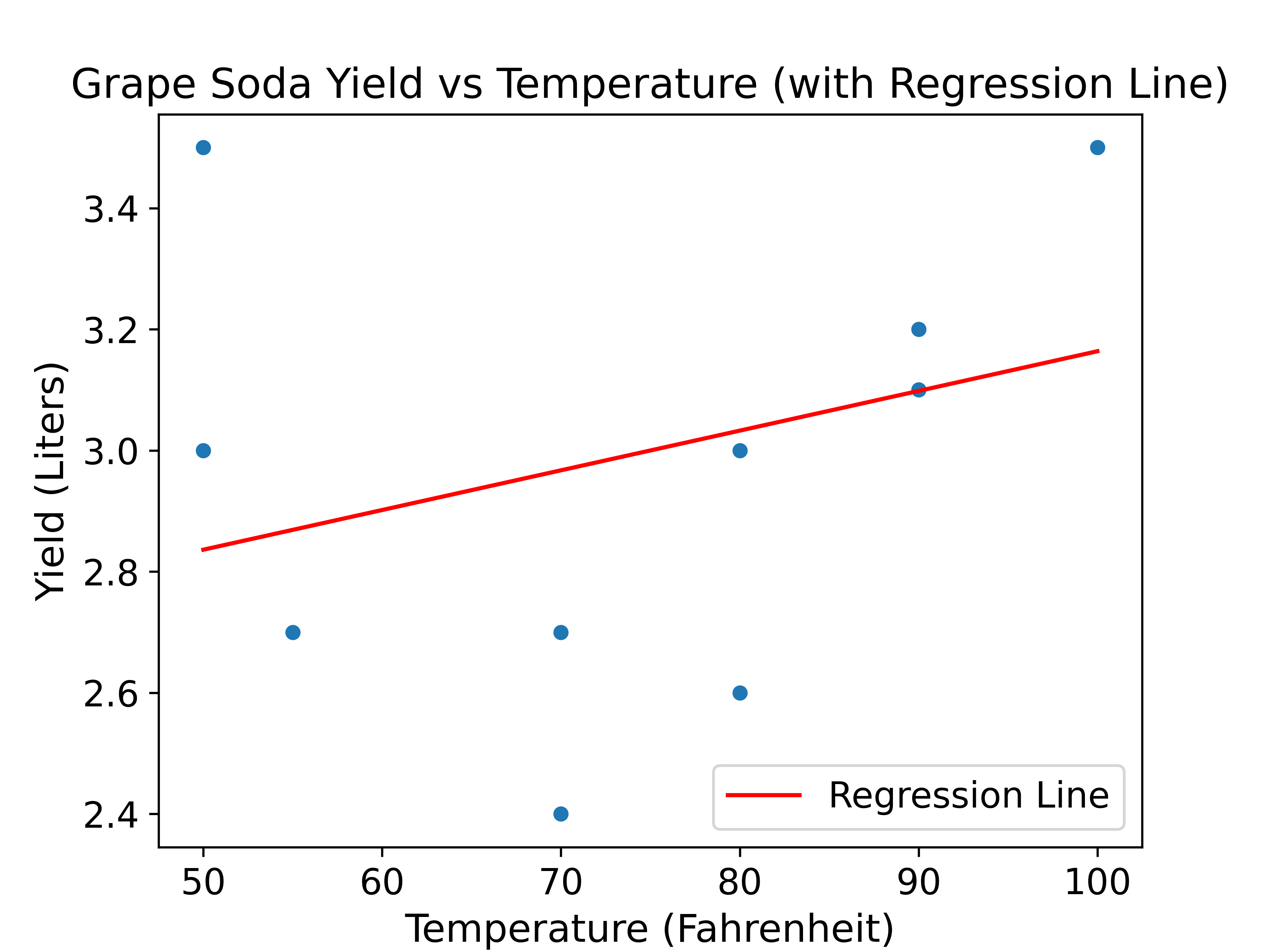
Given the above statistics, calculate the slope (\(\hat{\theta}_1\)) and y-intercept (\(\hat{\theta}_0\)) of the line of best fit using Mean Squared Error (MSE) as our loss function and :

\[ y = \hat{\theta}_0 + \hat{\theta}_1 x \]

Answer

\(\hat{\theta}_1 = r \frac{\sigma_y}{\sigma_x}\)

\(\hat{\theta}_1 = 0.5 \frac{0.3}{15} = 0.01\)

\(\hat{\theta}_0 = \bar{y} - \hat{\theta}_1 \bar{x}\)

\(\hat{\theta}_0 = 3 - 75.00*0.01 = 3 - 0.75 = 2.25\)

Note that the values of \(\sigma_y\) and \(\sigma_x\) are slightly different from what the table above shows, this was modified to make calculations slightly easier during discussion. This is why the intercept and slope of the line in the plot above do not match up exactly with the values we calculate.

---

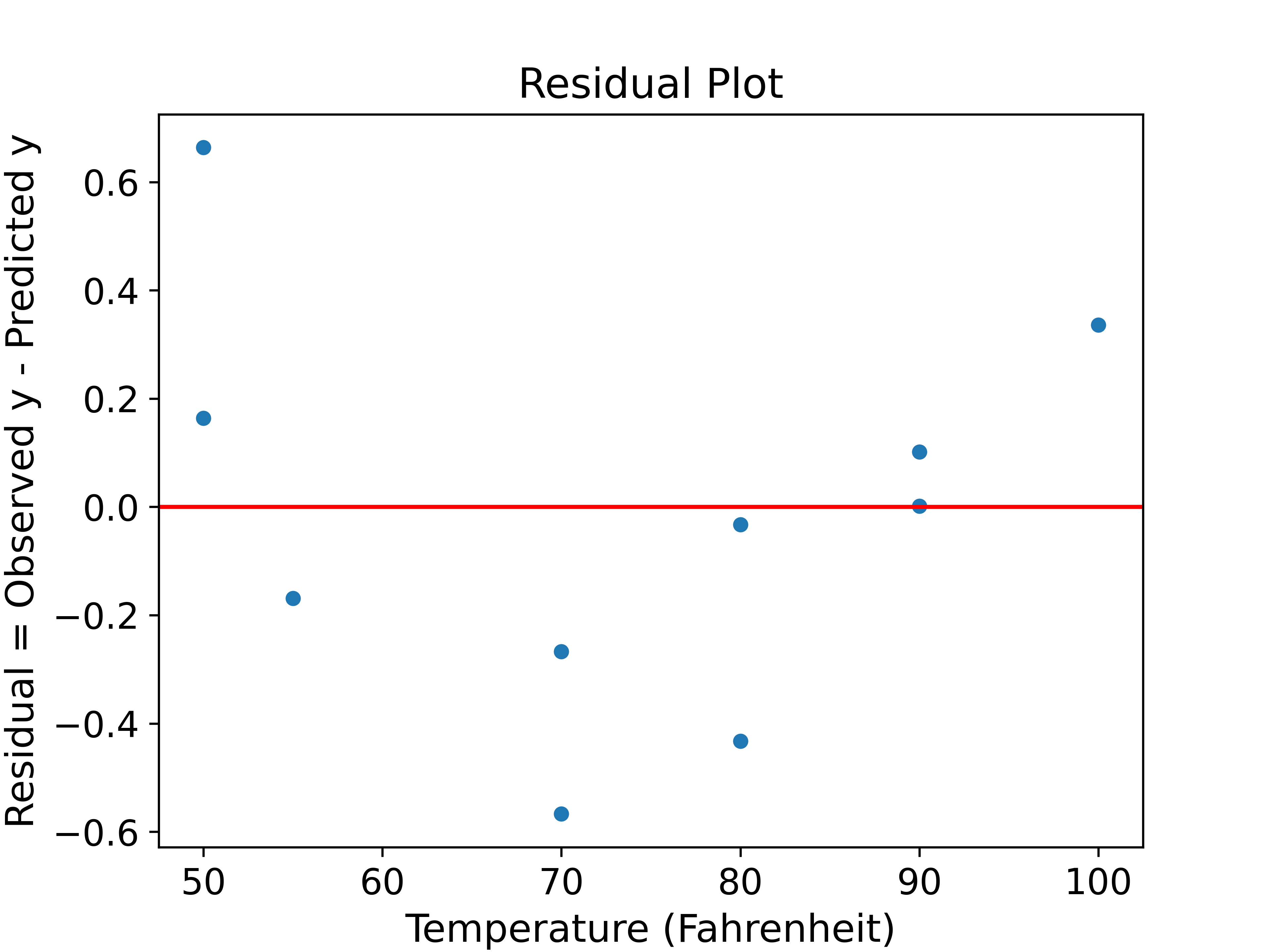
20.3.2 (b) (Extra)

Below, you can find a plot of the residuals from the line of best fit you calculated in part (a). What does the residual plot tell us about the relationship between x and y?

Answer

The plot of the residuals is not equally variable across all values of \(x\). This means that there is heteroscedasticity in our residuals. Thus, the relationship between \(x\) and \(y\) is likely not linear. \(y\) is likely not linear in terms of \(x\).

---

20.3.3 (c) (Extra)

Which of the following relations most closely represent the relationship we see between Temperature (\(x\)) and Yield (\(y\))?

• \(y = \theta_2 x^2\)
• \(y = \theta_2 x^2 + \theta_1 x + \theta_0\)
• \(y = \theta_1\log{x} + \theta_0\)
• \(y = \theta_1x + \theta_0\)

Answer

• \(y = \theta_2 x^2 + \theta_1 x + \theta_0\)

Based on the shape of the original and residual plots, we can see that the graph follows a curved, or quadratic (\(x^2\)), pattern as opposed to a linear one (\(x\)) or a logarithmic one (\(\log{x}\)). To choose between choice A or B, we can look at the intercept of the original graph; because all values have a yield above 2.4, we expect the intercept \(\theta_0\) to be a nonzero value, so we choose B instead of A.