36 Discussion 09: Bias & Variance (From Summer 2025)
36.1 Bias-Variance Trade-off
Your team would like to train a machine learning model to predict the next YouTube video a user will click on based on the videos the user has watched. We extract up to \(d\) attributes (such as length of video, view count, etc.) from each video, and our model will be based on the previous \(m\) videos watched by that user. Hence, the number of features for each data point for the model is \(m \times d\). Currently, you’re not sure how many videos to consider.
36.1.1 (a)
Your colleague, Lillian, generates the following plot, where the value \(d\) on the \(x\)-axis denotes the number of features used for a particular model. However, she forgot to label the \(y\)-axis. Assume that the features are added to the model in decreasing levels of importance: More important features are first, and less important ones are after.
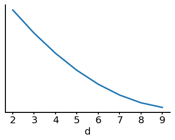
Which of the following could the \(y\)-axis represent? Select all that apply.
Answer
Training Error: Training error can decrease as we add more features.
Validation Error: This can be true depending on the underlying complexity of the data. In part (b), increasing \(d\) does not necessarily lower our validation error.
Bias: Decreases with increasing model complexity.
Variance: Increases with increasing model complexity.
When reviewing theoretical concepts like the bias-variance trade-off, keep the following in mind:
- Always be clear about conditions when answering questions—there are rarely absolute “always happens” statements because counter-examples exist. Be ready to explain these explicitly.
- Adding relevant features to a model can reduce training error, but adding irrelevant features may not. Stick to the rules, especially for exams where assumptions may change.
- When we refer to bias in solutions, we usually mean bias squared (bias\(^2\)), because bias itself can be positive or negative. In this context, “decreasing bias” doesn’t make literal sense.
- Variance typically increases with model complexity, though exceptions exist depending on the model type (beyond the scope of Data 100).
- Bias and variance are distinct concepts. They are combined in the bias-variance decomposition of MSE, but each has its own statistical meaning.
36.1.2 (b)
Lillian generates the following plot, where the value \(d\) is on the x-axis. However, she forgot to label the y-axis again.
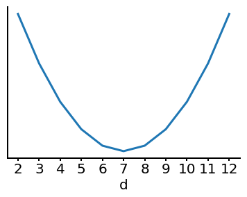
Which of the following could the y-axis represent? Select all that apply.
Answer
We can reason by the process of elimination. Under normal conditions, it can’t be the training error since the training error cannot begin to increase when adding model complexity. Bias also decreases with model complexity and variance increases with model complexity. This leaves validation error as the only option, giving \(d = 7\) as the optimal number of features to use.
A good question to consider here is: what is the best \(d\) value?
The answer is 7.
36.1.3 (c)
Explain what happens to the error on the holdout set as we increase \(d\). Why?
(Hint: The holdout set refers to a test set and not a validation set!)
Answer
For smaller \(d\), we are underfitting the training data since the model is less complex. The number of features we have does not allow us to fully understand the pattern and so our holdout error is high. As we increase \(d\), we have more features that allow us to pick up on some of the trends in the data and so the holdout error decreases a bit. However, there comes a point after which the features result in overfitting. Our model becomes more complex and does not seem to generalize as well to unseen data resulting in a high holdout error once again.36.2 More Bias-Variance Trade Off
We randomly sample \(n\) data points, \((x_i, y_i)\), and use them to fit a model \(f_{\hat\theta}(x)\) according to some procedure (e.g. OLS, Ridge, LASSO). Then, we sample a new data point (independent of our existing points) from the same underlying data distribution. Furthermore, assume that we have a function \(g(x)\), which represents the ground truth and \(\epsilon\), which represents random noise. \(\epsilon\) is produced by some noise generation process such that \(\mathbb{E}\left\lbrack\epsilon\right\rbrack = 0\) and \(\text{Var}(\epsilon)=\sigma^2\). Whenever we query \(Y\) at a given \(x\), we are given \(Y = g(x) + \epsilon\), a corrupted version of the real ground truth output. A new \(\epsilon\) is generated each time, independent of the last. We showed in the lecture that:
\[ \underbrace{\mathbb{E}\big[(Y - f_{\hat\theta}(x))^2\big]}_{} = \underbrace{\sigma^2}_{} + \underbrace{(g(x) - \mathbb{E}[f_{\hat\theta}(x)])^2}_{} + \underbrace{\mathbb{E}\big[(f_{\hat\theta}(x) - \mathbb{E}[f_{\hat\theta}(x)])^2\big]}_{} \]
This is a good time to make sure you understand what \(f_{\hat\theta}(x)\) means:
- We think of our predictions as functions of \(x\) parameterized by \(\hat{\theta}\).
- This is similar to \(\hat{y}_i\), but the notation \(f_{\hat\theta}(x)\) helps us see clearly where the randomness comes from (e.g., part (b) of the problem).
The noise term \(\epsilon\) is just a function used to generate a random number (often sampled from a normal distribution) with
\[\mathbb{E}[\epsilon] = 0 \quad \text{and} \quad \text{Var}(\epsilon) = \sigma^2.\]
This models random noise in the real world.
36.2.1 (a)
Label each of the terms above using the following word bank. Not all words will be used.
- observation variance
- model variance
- \((\text{observation bias})^2\)
- \((\text{model bias})^2\)
- model risk
- empirical mean square error
Answer
\[ \underbrace{\mathbb{E}[(Y - f_{\hat\theta}(x))^2]}_{\text{model risk}} = \underbrace{\sigma^2}_{\text{observation variance}} + \underbrace{(g(x) - \mathbb{E}[f_{\hat\theta}(x)])^2}_{(\text{model bias})^2} + \underbrace{\mathbb{E}\big[(f_{\hat\theta}(x) - \mathbb{E}[f_{\hat\theta}(x)])^2\big]}_{\text{model variance}} \]36.2.2 (b)
What quantities are random variables in the above equation? In our assumed data-generation process, where is the randomness in each variable coming from (i.e., which part of the assumed underlying model makes each random variable ‘random’)?
Answer
\(Y\) - this is the new observation at \(x\). Its randomness comes from the random noise \(\epsilon\).
\(f_{\hat\theta}\) - this is the model fitted from the data. Its randomness comes from sampling and the random noise \(\epsilon\).
\(\hat{\theta}\) - these are the optimal theta parameters. Like the model itself, the randomness stems from the sampling and the random noise \(\epsilon\).36.2.3 (c)
Calculate the value of \(\mathbb{E}[\epsilon \, f_{\hat\theta}(x')]\), where \(f_{\hat{\theta}}(x')\) is some predicted value of the response variable at some new fixed \(x'\) using a model trained on a random sample, and \(\epsilon\) is the observation error for a new data point at this fixed value of \(x'\).
Answer
Note that \(f_{\hat{\theta}}(x)\) is a random variable whose randomness comes from \(\hat{\theta}\) being random, which is itself random because of randomness in the training data. The data-generating mechanism for our new data point at \(x\) is independent of all the other data used to train our model by assumption, so we have that the sources of randomness for \(\epsilon\) and \(f_{\hat{\theta}}(x)\) are independent. Since \(\epsilon\) and \(\hat\theta\) are independent, \[\mathbb{E}[\epsilon f_{\hat\theta}(x)] = \mathbb{E}[\epsilon]\mathbb{E}[f_{\hat\theta}(x)]\]
And since \(\mathbb{E}[\epsilon] = 0\) by the definition we have given. Therefore, \[\mathbb{E}[\epsilon f_{\hat\theta}(x)] = \mathbb{E}[\epsilon]\mathbb{E}[f_{\hat\theta}(x)] = 0\]
Note that \(\epsilon\) here refers to the noise associated with our new data point \(x'\), which is independently drawn (as stated at the start of the question). This can seem a bit confusing since we’ve previously used \(\epsilon\) to refer to the noise associated with each of the data points, but it is used to simplify the notation. It might help to think of the noise associated with each of our points \(x_i\) as being \(\epsilon_i\) (which are i.i.d.), with the noise associated with \(x'\) as being \(\epsilon'\). It then becomes clearer why \(\epsilon'\) and \(f_{\hat\theta}(x)\) are independent.36.3 Regularization and Bias-Variance Trade-off
We will use a simple constant model \(f_\theta(x) = \theta\) to show the effects of regularization on bias and variance. For the sake of simplicity, we will assume that there is no noise or observational variance, so the ground truth output is equal to the observed outputs: \(Y = g(x)\).
36.3.1 (a)
Recall that the optimal solution for the constant model with an MSE loss and a dataset \(\mathcal{D}\) with \(y_1, y_2, ..., y_n\) is the mean \(\bar{y}\).
We use L2 regularization with a regularization penalty of \(\lambda > 0\) to train another constant model. Derive the optimal solution to this new constant model with L2 regularization to minimize the objective function below.
\[ R(\theta) = \arg \min_\theta \left[ \left( \frac{1}{n} \sum_{i=1}^n (y_i - \theta)^2 \right)+ \lambda \theta^2 \right] \] Note: As mentioned in the lecture, we do not impose a regularization penalty on the bias term and this problem only serves as a practice.
Answer
We use calculus to derive this result below:
\[\frac{dR}{d\theta} = \left( \frac{1}{n} \sum_i \frac{d}{d\theta} (y_i - \theta)^2 \right) + \lambda \frac{d}{d\theta}\theta^2 = \left( -\frac{2}{n} \sum_i (y_i - \theta) \right) + 2\lambda \theta\]
Set the derivative to 0, and solve for the optimal \(\hat{\theta}\).
\[ \left( -\frac{2}{n}\sum_i (y_i - \hat{\theta}) \right) + 2\lambda \hat{\theta} = 0 \implies \left( -\frac{1}{n}\sum_i y_i \right) + \hat{\theta} + \lambda \hat{\theta} = 0 \]
The optimal \(\hat{\theta}\) is:
\[\frac{1}{n}\sum_i y_i = \hat{\theta} (1+\lambda)\]
\[ \hat{\theta} = \frac{1}{n(1 + \lambda)} \sum_i y_i = \frac{1}{1 + \lambda} \bar{y} \]
It can be tricky to know how to handle a hyper-parameter like \(\lambda\) in an optimization problem.
- Treat hyper-parameters as constants when differentiating with respect to other variables—there’s nothing to worry about.
- Notice the presence of \(\lambda\) in the solution. For example:
- As \(\lambda \to 0\), the solution reduces to the standard MSE case (the observation mean).
- When \(\lambda > 0\), the regularized MSE solution is not the mean. Regularization shifts the solution, and the magnitude of \(\theta\) is smaller since \(\frac{1}{1 + \lambda} < 1\).
- As \(\lambda \to 0\), the solution reduces to the standard MSE case (the observation mean).
This is a concrete example of how regularization decreases model complexity.
36.3.2 (b) (Extra)
Use the bias-variance decomposition to show that for a constant model without regularization, its optimal expected loss on a sample test point \((x, Y)\) in terms of the training data \(y\) is equal to the following.
\[\mathbb{E}_\mathcal{D}[(Y - f_{\hat\theta}(x))^2] = (Y - \mathbb{E}_\mathcal{D}[\bar{y}])^2 + \text{Var}_\mathcal{D}(\bar{y})\]
Note: The subscript next to the expectation and variance lets you know what is random inside the expectation (i.e., what is the expectation taken over?). In this case, we calculate the expectation and variance of \(\bar{y}\) across the dataset \(\mathcal{D}\).
Answer
Starting from the bias-variance decomposition presented in the lecture: \[\mathbb{E}[(Y - f_{\hat\theta}(x))^2] = \sigma^2 + (g(x) - \mathbb{E}[f_{\hat\theta}(x)])^2 + \text{Var}(f_{\hat\theta}(x))\]
Recall that we are not dealing with any noise (\(\epsilon \sim \mathbb{N}(0, 0)\)), so we can eliminate the \(\sigma^2\) term. Then, \(g(x) = Y\), so we can replace all instances of \(g(x)\) with \(Y\).
\[\mathbb{E}[(Y - f_{\hat\theta}(x))^2] = (Y - \mathbb{E}[f_{\hat\theta}(x)])^2 + \text{Var}(f_{\hat\theta}(x))\]
We can then derive \(f_{\hat\theta}(x)\) using the assumptions of our constant model. We know that \(f_{\hat\theta}(x) = \bar{y}\). We simplify the following expressions:
\[\mathbb{E}[(Y - f_{\hat\theta}(x))^2] = (Y - \mathbb{E}[\bar{y}])^2 + \text{Var}(\bar{y})\]
Note that we omit the subscript \(\mathcal{D}\) is omitted in the above equations as it is clear we are working with that dataset.36.3.3 (c)
Use the bias-variance decomposition to show that for a constant model with L2 regularization, its optimal expected loss on a sample test point \((x, Y)\) in terms of the training data \(y\) is equal to the following.
\[\mathbb{E}_\mathcal{D}[(Y - f_{\hat\theta}(x))^2] = (Y - \frac{1}{1 + \lambda} \mathbb{E}_\mathcal{D}[\bar{y}])^2 + \frac{1}{(1 + \lambda)^2} \text{Var}_\mathcal{D}(\bar{y})\]
What expected loss do we obtain when \(\lambda=0\), and what does that mean in terms of our model?
Note: The subscript next to the expectation and variance lets you know what is random inside the expectation (i.e., what is the expectation taken over?). In this case, we calculate the expectation and variance of \(\bar{y}\) across the dataset \(\mathcal{D}\).
Answer
Starting from the bias-variance decomposition presented in the lecture: \[\mathbb{E}[(Y - f_{\hat\theta}(x))^2] = \sigma^2 + (g(x) - \mathbb{E}[f_{\hat\theta}(x)])^2 + \text{Var}(f_{\hat\theta}(x))\]
Recall that we are not dealing with any noise (\(\epsilon \sim \mathbb{N}(0, 0)\)), so we can eliminate the \(\sigma^2\) term. Then, \(g(x) = Y\), so we can replace \(g(x)\) with \(Y\).
\[\mathbb{E}[(Y - f_{\hat\theta}(x))^2] = (Y - \mathbb{E}[f_{\hat\theta}(x)])^2 + \text{Var}(f_{\hat\theta}(x))\]
We can then derive \(f_{\hat\theta}(x)\) using the assumptions of our constant model. We know that \(f_{\hat\theta}(x) = \frac{1}{1 + \lambda}\bar{y}\). We simplify the following expressions:
\[\mathbb{E}[(Y - f_{\hat\theta}(x))^2] = (Y - \mathbb{E}[\frac{1}{1 + \lambda}\bar{y}])^2 + \text{Var}(\frac{1}{1 + \lambda}\bar{y})\]
We can simplify:
\[\mathbb{E}[(Y - f_{\hat\theta}(x))^2] = (Y - \frac{1}{1 + \lambda} \mathbb{E}[\bar{y}])^2 + \frac{1}{(1 + \lambda)^2} \text{Var}(\bar{y})\]
Setting \(\lambda=0\) is equivalent to using a constant model without L2 regularization, and we get the following equation for the expected loss:
\[\mathbb{E}[(Y - f_{\hat\theta}(x))^2] = (Y - \mathbb{E}[\bar{y}])^2 + \text{Var}(\bar{y})\]36.3.4 (d)
Remark on how regularization has affected the model bias and variance as \(\lambda\) increases. Consider what would happen to these quantities as \(\lambda \to \infty\).
Answer
The model bias has increased since the gap between a test point \(Y\) and a scaled ``best estimate’’ value is likely larger than between the test point and the actual best estimate. As \(\lambda \to \infty\), the model bias squared will tend towards \(Y^2\).
The model variance has decreased since \(\frac{1}{(1 + \lambda)^2}\) if \(\lambda > 0\) will always be less than 1. Hence, our variance compared to the vanilla bias-variance decomposition from part (b) is reduced by a factor greater than 1. As \(\lambda \to \infty\), the model variance will become 0.