40 Discussion 13: PCA & Clustering (From Summer 2025)
The notation used for PCA starting from Spring 2024 differs from previous semesters a bit.
- Principal Component: The columns of \(V\). These vectors specify the principal coordinate system and represent the directions along which the most variance in the data is captured.
- Latent Vector Representation of X: The projection of our data matrix \(X\) onto the principal components, \(Z = XV = US\) (as denoted in lecture). The columns of \(Z\) are called latent factors or component scores. In previous semesters, the terminology was different and this was termed the principal components of \(X\).
- \(S\) (as in SVD): The diagonal matrix containing all the singular values of \(X\).
- \(\Sigma\): The covariance matrix of \(X\). Assuming \(X\) is centered, \(\Sigma = \frac{1}{n} X^T X\). In previous semesters, the singular value decomposition of \(X\) was written out as \(X=U \Sigma V^T\), but we now use \(X=USV^T\). Note the difference between \(\Sigma\) in that context compared to this semester.
40.1 PCA Basics
Consider the following dataset, where \(X\) is the corresponding \(4 \times 3\) design matrix. The mean and variance for each of the features are also provided.
| Observations | Feature 1 | Feature 2 | Feature 3 |
|---|---|---|---|
| 1 | -3.59 | 7.39 | -0.78 |
| 2 | -8.37 | -5.32 | 0.90 |
| 3 | 1.75 | -0.61 | -0.62 |
| 4 | 10.21 | -1.46 | 0.50 |
| Mean | 0 | 0 | 0 |
| Variance | 47.56 | 21.35 | 0.51 |
40.1.1 (a)
Recall that we define the columns of \(V\) as the principal components. By projecting \(X\) onto the principal components (i.e. computing \(XV\)), we can construct the latent vector representation of \(X\). Alternatively, you can also calculate the latent vector representation using \(US\). Using \(X=USV^T\) prove that \(XV = US\).
Answer
Since \(V\) is orthonormal, we know that \(V^TV = I\). Starting with \(X = U S V^T\), we right multiply by \(V\) on both sides: \[ XV = U S V^TV = U S I = U S \] This completes the proof.The matrices from the Singular Value Decomposition (\(X = USV^T\)) have special properties that make them incredibly useful in data analysis.
- \(U\) and \(V\) (The Orthonormal Matrices): Both \(U\) and \(V\) are orthonormal matrices. This means their columns are mutually perpendicular unit vectors. The most powerful consequence of this property is that the inverse of an orthonormal matrix is simply its transpose. For the matrix \(V\), this means \(V^{-1} = V^T\). This makes many calculations, like solving for the latent vector representation (\(XV = US\)), computationally efficient.
- The columns of \(V\) are the principal components, which represent the directions of maximum variance in your data.
- \(S\) (The Diagonal Matrix): The matrix \(S\) is a diagonal matrix, meaning all of its off-diagonal elements are zero. Its diagonal entries are the singular values of the data, sorted from largest to smallest. Each singular value corresponds to a principal component and represents its “magnitude” or importance in capturing the data’s variance.
40.1.2 (b)
Compute the projection of \(X\) onto the first principal component, also called the first latent factor (round to 2 decimal places).
Answer
We compute the first latent factor by multiplying \(X\) by the first row of \(V^T\) to get \(\approx \begin{bmatrix} -3.44 & -8.47 & 1.74 & 10.18 \end{bmatrix}^T\) (your values may differ slightly due to rounding).
You can also compute the first latent factor by observing that \(XV = U S\). Therefore, the first latent factor is also the first column of \(U S\).40.1.3 (c)
What is the component score of the first principal component? In other words, how much of the total variance of \(X\) is captured by the first principal component?
Answer
The variance captured by \(i\)-th principal component of the original data \(X\) is equal to \[\frac{(i\text{-th singular value})^2}{\text{number of observations } n}\]
In this case, \(n = 4\), and \(s_1 = 13.79\). Therefore, the component score can be computed as follows:
\[\frac{13.79^2}{4} = 47.54\]40.1.4 (d)
(Bonus) Given the results of (a), how can we interpret the rows of \(V^T\)? What do the values in these rows represent?
Answer
The rows of \(V^T\) are the same as the columns of \(V\) which we know are the principal components of X. Each latent factor of \(X\) is a linear combination of \(X\)’s features. The rows of \(V^T\) correspond to the weights of each feature in the linear combinations that make up their respective latent factors.40.2 Applications of PCA
Minoli wants to apply PCA to food_PCA, a dataset of food nutrition information to understand the different food groups.

She needs to preprocess her current dataset in order to use PCA.
40.2.1 (a)
Which of the following are appropriate preprocessing steps when performing PCA on a dataset?
Answer
40.2.2 (b)
Assume you have correctly preprocessed your data using the correct response in part (a). Write a line of code that returns the first 3 latent factors assuming you have the correctly preprocessed food_PCA and the following variables returned by SVD.
u, s, vt = np.linalg.svd(food_PCA, full_matrices = False)
first_3_latent_factors = ________________________________
Answer
u, s, vt = np.linalg.svd(food_PCA, full_matrices = False)
first_3_latent_factors = food_PCA @ vt.T[:, :3]
Note that @ is how matrix multiplication is carried out in Python.
Alternatively, we can also multiply the first 3 columns of \(U\) and \(S\):
u, s, vt = np.linalg.svd(food_PCA, full_matrices = False)
first_3_latent_factors = u[:, :3] * s[:3]
40.2.3 (c)
The scree plot below depicts the proportion of variance captured by each principal component.
Which of the following lines of code could have created the plot above?
Answer
NumPy operations, we can calculate the \(y\)-values as s**2/np.sum(s**2). The corresponding \(x\)-values should run from 1 to the number of columns of food_PCA, which gives us np.arange(1, food_PCA.shape[1]+1).
40.2.4 (d)
Using the elbow method, how many principal components should we choose to represent the data?
Answer
The elbow of a scree plot is the point where adding more principal components results in diminishing returns. In other words, we look for the “elbow” in the curve just before the line flattens out. This point is at PC 3 in the graph above, so we choose 3 as the number of principal components. Note that not all scree plots will have an obvious elbow.40.3 Interpreting PCA Plots
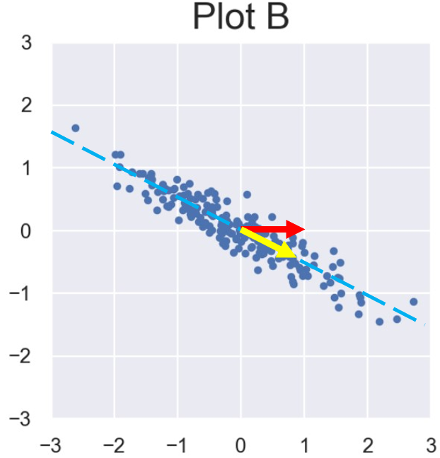
Xiaorui has three datasets \(A\), \(B\), and \(C \in \mathbb{R}^{100 \times 2}\). That is, each dataset consists of 100 data points in two dimensions. He visualizes the datasets using scatterplots, labeled Plot A, Plot B, and Plot C, respectively:

40.3.1 (a)
If he applies PCA to each of the above datasets and uses only the first principal component, which dataset(s) would have the lowest reconstruction error? Select all that apply.
Answer
Most of the variance in Plot B lies roughly about a single line. The variance captured by the second PC is far smaller in Plot B compared to plots A and C. In both Plot A and Plot C, there are significant amounts of variance in two orthogonal directions, so PC1 would not be able to capture as much of the total variance.
Since we want to have the lowest reconstruction error while using only 1 PC, we pick Plot B.40.3.2 (b)
If he applies PCA to each of the above datasets and uses the first two principal components, which dataset(s) would have the lowest reconstruction error? Select all that apply.
Answer
40.3.3 (c)
Suppose he decides to take the Singular Value Decomposition (SVD) of one of the three datasets, which we will call Dataset \(X\). He runs the following piece of code:
X_bar = X - np.mean(X, axis=0)
U, S, V_T = np.linalg.svd(X_bar)
He gets the following output for \(S\):
array([15.59204498, 3.85871854])and the following output for \(V^T\):
array([[0.89238775, -0.45126944], [0.45126944, 0.89238775]])Based on the given plots and the SVD, which of the following datasets does Dataset X most closely resemble? Select one option.
Answer
40.4 Clustering
40.4.1 (a)
Describe the difference between clustering and classification.
Answer
Both involve assigning arbitrary classes to each observation. In classification, we have a labeled training set, i.e. a ground truth we can use to train our model. In clustering, we have no ground truth, and are instead looking for patterns in unlabeled data. Classification falls under supervised machine learning because it is concerned with predicting the correct/specific class given the true labels to the data. Clustering falls under unsupervised machine learning because there are no provided “true” labels - instead it is concerned with the patterns across the data (rather than where the data belongs).40.4.2 (b)
Given a set of points and their labels (or cluster assignments) from a K-Means clustering, how can we compute the centroids of each of the clusters?
Answer
For each label, find the mean of all of the data points corresponding to that label. In other words, compute centroids \(c_i\) for each label/cluster’s set of data points \(L_i\) and corresponding data points \(x_j \in L_i\): \[ c_i = \frac{1}{n} \sum_{x_j \in L_i} x_j \]40.4.3 (c)
Describe qualitatively what it means for a data point to have a negative silhouette score.
Answer
The silhouette score of a data point is negative if it is on average closer to the points in the neighboring cluster than its own cluster.40.4.4 (d)
Suppose that no two points have the same distance from each other. Are the cluster labels computed by K-means always the same for a given dataset? What about for max agglomerative clustering?
Answer
The cluster labels computed by K-means could be different if we change the initial centers. This cannot happen for max agglomerative clustering because every point starts in its own cluster, and there is no choice involving initialization.Congrats!!!
You completed the last discussion question for Data 100! I hope you found my discussions useful and that you succeed on the final. The content you’ve learned in the course is useful for both industry data analysis jobs and advanced courses like CS 189, Data 101, or Data 102. I hope you have a wonderful semester and a great break after the final, and I hope to see you somewhere on campus!