1 Data 102 Discussion 01: Bayes’ Rule & Binary Decisions
1.0.1 Contact Information
| Name | Wesley Zheng |
| Pronouns | He/him/his |
| wzheng0302@berkeley.edu | |
| Discussion | Wednesdays, 11–12 PM @ Wheeler 224 |
| Office Hours | Tuesdays, 9–10 AM & 11-12 PM @ Gateway B1040 |
Contact me by email at ease — I typically respond within a day or so!
1.1 Bayes’ Rule Review
Bayes’ rule lets us update beliefs about a hidden cause after observing data. It will show up throughout this course whenever we go from likelihoods and priors to posteriors.
Law of Total Probability
If events \(A_1, \ldots, A_k\) partition the sample space, \[ \mathbb{P}(B) = \sum_{i=1}^{k} \mathbb{P}(B \mid A_i)\, \mathbb{P}(A_i). \]
Bayes’ Rule
\[ \mathbb{P}(A \mid B) = \frac{\mathbb{P}(B \mid A)\, \mathbb{P}(A)}{\mathbb{P}(B)}. \]
- \(\mathbb{P}(A)\) = prior
- \(\mathbb{P}(B \mid A)\) = likelihood
- \(\mathbb{P}(A \mid B)\) = posterior
- \(\mathbb{P}(B)\) = marginal (often expanded with the law of total probability)
Tip: When the question asks for \(\mathbb{P}(\text{cause} \mid \text{observation})\), reach for Bayes. When it asks for \(\mathbb{P}(\text{observation})\) with multiple possible causes, use total probability first.
There are two boxes, the odd box containing \(1\) black marble and \(3\) white marbles, and the even box containing \(2\) black marbles and \(4\) white marbles. A box is selected at random, and a marble is drawn at random from the selected box.
This warm-up is meant to refresh Bayes’ rule, which shows up throughout the worksheet and later assignments. Take a moment to make sure the law of total probability and Bayes’ rule feel comfortable before moving on.
1.1.1 (a)
What is the probability that the marble is black?
Answer
\[\frac{7}{24}\]
\[ \mathbb{P}(\text{B}) = \mathbb{P}(\text{B} \mid \text{Odd}) \mathbb{P}(\text{Odd}) + \mathbb{P}(\text{B}\mid \text{Even}) \mathbb{P}(\text{Even})= \frac{1}{4} \times \frac{1}{2} + \frac{2}{6} \times \frac{1}{2} = \frac{7}{24}\]
1.1.2 (b)
Given the marble is white, what is the probability that it came from the even box?
Answer
\[\frac{8}{17}\]
By Bayes’ Rule, we know that: \[\begin{align*} \mathbb{P}(\text{Even} \mid \text{W}) & = \frac{\mathbb{P}(\text{W} \mid \text{Even}) \mathbb{P}(\text{Even})}{\mathbb{P}({\text{W}})} \\ & = \frac{\mathbb{P}(\text{W} \mid \text{Even}) \mathbb{P}(\text{Even})}{1 - \mathbb{P}({\text{B}})} \\ & = \frac{\frac{4}{6} \times \frac{1}{2}} {1 - \frac{7}{24}} = \frac{8}{17} \end{align*}\]
1.2 Consequences of Binary Decisions
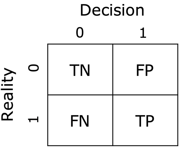
Binary decisions compare a decision \(D \in \{0,1\}\) to a reality \(R \in \{0,1\}\). Outcomes fill a \(2 \times 2\) table: TP, FP, FN, TN.
Row-wise rates (conditional on reality):
- True Positive Rate / Sensitivity / Power: \[ \text{TPR} = \frac{\text{TP}}{\text{TP} + \text{FN}} = \mathbb{P}(D=1 \mid R=1) \]
- False Positive Rate / Type I error rate: \[ \text{FPR} = \frac{\text{FP}}{\text{FP} + \text{TN}} = \mathbb{P}(D=1 \mid R=0) \]
- True Negative Rate / Specificity: \[ \text{TNR} = \frac{\text{TN}}{\text{TN} + \text{FP}} = \mathbb{P}(D=0 \mid R=0) = 1 - \text{FPR} \]
Column-wise rates (conditional on the decision):
- False Discovery Proportion: \[ \text{FDP} = \frac{\text{FP}}{\text{FP} + \text{TP}} = \mathbb{P}(R=0 \mid D=1) \]
- False Omission Proportion: \[ \text{FOP} = \frac{\text{FN}}{\text{FN} + \text{TN}} = \mathbb{P}(R=1 \mid D=0) \]
Common pitfall: \(\text{FPR} \neq 1 - \text{TPR}\) in general — they condition on different rows of the table.
In the first lecture, we discussed binary decision making. The results of binary decisions can be summarized by the \(2 \times 2\) table below:
Indicate whether each of the following statements are True or False.
1.2.1 (a)
\(\text{FPR} = 1 - \text{TPR}\), where FPR and TPR and the False Positive Rate and True Positive Rate respectively.
Answer
False.
Recall that by definition, \[\begin{align*} \text{FPR} = \frac{{\rm FP}}{{\rm FP} + {\rm TN}} \\ \text{TPR} = \frac{{\rm TP}}{{\rm FN} + {\rm TP}} \end{align*}\] We want to see if \(\text{FPR} = 1 - \text{TPR}\). Plugging in the definitions, we have: \[\begin{align*} \frac{{\rm FP}}{{\rm FP} + {\rm TN}} &= 1 - \frac{{\rm TP}}{{\rm FN} + {\rm TP}} \\ \frac{{\rm FP}}{{\rm FP} + {\rm TN}} &= \frac{{\rm FN} + {\rm TP}}{{\rm FN} + {\rm TP}} - \frac{{\rm TP}}{{\rm FN} + {\rm TP}} \\ \frac{{\rm FP}}{{\rm FP} + {\rm TN}} &\neq \frac{{\rm FN}}{{\rm FN} + {\rm TP}} \end{align*}\]
1.2.2 (b)
\(\text{Specificity} = 1 - \text{FPR}\).
Answer
True.
Sensitivity and specificity are equivalent to True Positive Rate (TPR) and True Negative Rate (TNR), respectively. Thus, \[\begin{align*} \text{Specificity} &= \text{TNR} \\ & = \frac{\text{TN}}{\text{TN} + \text{FP}} \\ & = \frac{\text{TN} + \text{FP} - \text{FP}}{\text{TN} + \text{FP}} \\ & = 1 - \frac{\text{FP}}{\text{TN} + \text{FP}} \\ & = 1 - \text{FPR}. \end{align*}\]
1.2.3 (c)
The False Discovery Proportion (FDP) can be thought of as the conditional probability that the reality is null (\(R=0\)), given that a discovery was made (\(D=1\)).
Answer
True.
\[\text{FDP} = \frac{{\rm FP}}{{\rm FP} + {\rm TP}} = \mathbb{P}(R=0 \mid D=1)\] In words, FDP represents the proportion of times a model’s decision of \(1\) was incorrect out of all the times the model predicted \(1\).
1.2.4 (d)
Define the False Omission Proportion (FOP) as \(\frac{\text{FN}}{\text{FN} + \text{TN}}\). This is a column-wise rate. Additionally, in your own words, describe what the FOP measures.
Answer
True.
Column-wise rates can be thought of as conditional probabilities of reality given a fixed decision. The FOP measures the proportion of false negatives to all negative predictions. Since FOP only considers the data points which correspond to negative predictions, the FOP is a column-wise rate. Visually, we can see that FN and TN both appear in the same column of the \(2 \times 2\) table.
1.3 COVID-19 Testing
Sensitivity and specificity are row-wise rates. FDP is a column-wise rate, so we need Bayes’ rule (and prevalence) to convert between them.
Given:
- \(\text{Sensitivity} = \mathbb{P}(D=1 \mid R=1) = \text{TPR}\)
- \(\text{Specificity} = \mathbb{P}(D=0 \mid R=0) = 1 - \text{FPR}\)
- \(\text{Prevalence} = \pi_1 = \mathbb{P}(R=1)\)
Bayes gives: \[ \text{FDP} = \mathbb{P}(R=0 \mid D=1) = \frac{(1-\text{specificity})(1-\pi_1)}{(1-\text{specificity})(1-\pi_1) + (\text{sensitivity})\,\pi_1}. \]
An equivalent rearranged form from lecture: \[ \text{FDP} = \frac{1}{1 + \dfrac{\text{TPR}}{\text{FPR}} \cdot \dfrac{\pi_1}{1-\pi_1}}. \]
Intuition: Holding the test fixed, lower prevalence \(\Rightarrow\) higher FDP. Rare events make false positives a larger share of all positive calls.
A large study of \(80{,}000\) COVID-19 rapid tests over 2.5 years found that they have a sensitivity of \(34.5\%\) and a specificity of \(99.6\%\)1.
1.3.1 (a)
Calculating FDP I
Some estimates put the current number of COVID-19 cases (as of January 22) in the USA at about 5.6 million, out of a population of about 341 million. If this is the case, what would the FDP for a rapid test be? Assume that the test is performed on an individual drawn uniformly at random from the US.
Answer
\[\approx 0.41\]
From the question, we are told: \[\begin{align*} \text{Sensitivity} &= \mathbb{P}(D=1 \mid R=1)=0.345 \\ \text{Specificity} &= \mathbb{P}(D=0 \mid R=0)=0.996 \\ \text{Prevalence} &= \mathbb{P}(R=1) = \pi_1 = \frac{5600000}{341000000} = 0.0164 \end{align*}\] By definition, \(\text{FDP} = \mathbb{P}(R=0 \mid D=1)\). We can use Bayes’ rule just as we did in lecture: \[\begin{align*} \mathbb{P}(R=0 \mid D=1) &= \frac{\overbrace{\mathbb{P}(D=1 \mid R=0)}^{1-\text{specificity}}\mathbb{P}(R=0)}{\underbrace{\mathbb{P}(D=1 \mid R=0)}_{1-\text{specificity}}\mathbb{P}(R=0) + \underbrace{\mathbb{P}(D=1 \mid R=1)}_{\text{sensitivity}}\mathbb{P}(R=1)} \\ &= \frac{(1-0.996)(1-0.0164)}{(1-0.996)(1-0.0164) + 0.345\cdot 0.0164} \\ &\approx 0.41 \end{align*}\] You could also have used the rearranged formula from lecture: \[\begin{align*} \text{FDP} &= \frac{1}{1 + \frac{{\rm TPR}}{{\rm FPR}} \cdot \frac{\pi_1}{1-\pi_1}} \\ &= \frac{1}{1 + \frac{0.345}{1-0.996} \cdot \frac{0.0164}{1-0.0164}} \\ &\approx 0.41 \end{align*}\]
1.3.2 (b)
Calculating FDP II
Suppose that instead of considering an individual drawn uniformly at random from the entire population, we consider someone who is sick and is motivated to take a rapid test. Given that several flu variants and RSV are also circulating, we’ll assume they have a \(1/3\) chance of having COVID-19.
Assuming this is the true prevalence for people who take rapid tests, what is the FDP?
Answer
\[\approx 0.02\]
Now, our prevalence has changed: \[\text{Prevalence} = \mathbb{P}(R=1) = \pi_1 = 1/3 \approx 0.333\] We can recompute the FDP by plugging in the new prevalence in either formula shown in the solution to (a) (the rearranged formula is easier here): \[\begin{align*} \text{FDP} &= \frac{(1-0.996)(2/3)}{(1-0.996)(2/3) + 0.345\cdot 1/3} \\ \text{FDP} &= \frac{1}{1 + \frac{0.345}{1-0.996} \cdot \frac{1/3}{2/3}} \\ &\approx 0.02 \end{align*}\]
1.3.3 (c)
Connecting Prevalence and FDP
Compare the FDPs calculated in (a) and (b). How does prevalence affect FDP? Why does this make intuitive sense?
Answer
A lower prevalence corresponds to a higher FDP.
In (b), when the prevalence of COVID increased from 5.6 million per 341 million (or around 16 per 1000) to \(1/3\), the FDP drastically decreased from about 41% to 2%. So a lower prevalence corresponds to a higher FDP. This makes intuitive sense: when very few people have COVID, we’ll have fewer positive tests total, and more of them will be mistakes (false positives).
SARS-CoV-2 antigen rapid detection tests: test performance during the COVID-19 pandemic and the impact of COVID-19 vaccination. Wagenhauser et al. eBioMedicine, Volume 109, 105394.↩︎