2 Data 102 Discussion 02: Hypothesis Testing & ROC Curves
2.0.1 Contact Information
| Name | Wesley Zheng |
| Pronouns | He/him/his |
| wzheng0302@berkeley.edu | |
| Discussion | Wednesdays, 11–12 PM @ Wheeler 224 |
| Office Hours | Tuesdays, 9–10 AM & 11-12 PM @ Gateway B1040 |
Contact me by email at ease — I typically respond within a day or so!
2.1 Hypothesis Testing
In binary hypothesis testing we choose a point on the ROC by trading off two rates:
- Significance level \(\alpha = \mathbb{P}(\text{Reject } H_0 \mid H_0) = \text{FPR}\)
- Power \(= \mathbb{P}(\text{Reject } H_0 \mid H_a) = \text{TPR}\)
Neyman–Pearson strategy: fix the largest FPR you are willing to tolerate (\(\alpha\)), then maximize power among all tests with level at most \(\alpha\).
Likelihood-ratio test (most powerful level-\(\alpha\) test): \[ \delta(x)=\begin{cases} \text{Reject } H_0 & : & \dfrac{f(x;\,\theta_a)}{f(x;\,\theta_0)} > \eta \\ \text{Accept } H_0 & : & \dfrac{f(x;\,\theta_a)}{f(x;\,\theta_0)} \leq \eta \end{cases} \] where \(\eta\) is chosen so that \(\mathbb{P}(\delta(x)=1 \mid H_0)=\alpha\).
One can imagine different metrics for quantifying how “good” a decision is. For example, we would like our decisions to have both high true positive rate and low false positive rate. Our goal as statisticians is to develop reasonable strategies for doing well on both metrics. In other words, how should we pick a point on the ROC curve? Once we pick a point, how do we achieve it?
The Neyman-Pearson Lemma offers one solution, in the case of hypothesis testing. We call the probability of a false positive under null hypothesis, \(H_0\), the significance level of a test and we call the probability of a true positive under the alternative hypothesis, \(H_a\), the power of a test.
The Neyman-Pearson formulation makes the following recommendation: fix a false positive rate you are willing to tolerate, then pick the point on the ROC curve which maximizes power. The Neyman-Pearson Lemma prescribes how to achieve this point by selecting an appropriate test statistic, the likelihood ratio:
Lemma (Neyman & Pearson, 1933) For any significance level \(\alpha \in [0, 1]\), the following likelihood-ratio test maximizes power among all tests with level at most \(\alpha\): \[ \delta(x)=\begin{cases} \text{Reject Null } (1) & : & \dfrac{f(x; \, \theta_a)}{f(x; \, \theta_0)} > \eta \\ \textit{Accept Null } (0) & : & \dfrac{f(x; \, \theta_a)}{f(x; \, \theta_0)} \leq \eta \end{cases} \] where \(x\) is the observed data, \(\delta(x)\) indicates the decision made, \(f(\cdot; \, \theta_0), f(\cdot; \, \theta_a)\) are the likelihoods under the null and alternative distributions respectively, and \(\eta\) is the real value such that \(\mathbb{P}(\delta(x) = 1 \mid H_0) = \alpha\).
Let’s try an example where you will apply the Neyman-Pearson Lemma. Suppose that you have a sample from a distribution with probability density function \(f(x; \, \theta)=\theta x^{\theta-1}\) where \(0<x<1\). You would like to design a test to discern between the null hypothesis that \(\theta=3\), and the alternative hypothesis that \(\theta=4\).
2.1.1 (a)
Deriving a Likelihood Ratio Test
Derive the most powerful test for this problem such that the significance level is less than \(\alpha\). Solve for \(\eta\), then state the decision criteria in terms of the likelihood ratio.
Answer
\[ \delta(x)=\begin{cases} \text{Reject Null} & : & \dfrac{f(x; \, \theta_a)}{f(x; \, \theta_0)} > \dfrac{4}{3} (1 - \alpha)^{1/3} \\ \text{Accept Null} & : & \dfrac{f(x; \, \theta_a)}{f(x; \, \theta_0)} \leq \dfrac{4}{3} (1 - \alpha)^{1/3} \end{cases} \]
Leveraging the Neyman-Pearson Lemma, we design a likelihood-ratio test. The likelihood ratio has the form: \[ \frac{f(x; \, \theta_a)}{f(x; \, \theta_0)} = \frac{4 x^{3}}{3 x^{2}}=\frac{4x}{3}. \]
Now, following the lemma, we need to solve for \(\eta\) such that the test has significance level \(\alpha\). In other words, we want to find \(\eta\) such that \[ \begin{align*} \text{FPR} &= \mathbb{P}( D = 1 \mid R = 0) && \text{(lecture notation)} \\ &= \mathbb{P}( \delta(x) = 1 \mid H_0) && \text{(lemma notation)} \\ &= \mathbb{P} \left( \frac{4x}{3} > \eta \mid H_0 \right) = \alpha. \end{align*} \]
To solve for \(\eta\), note that \[ \mathbb{P}\left( \frac{4x}{3} > \eta \mid H_0 \right) = \alpha \] \[ \mathbb{P}\left( x > \frac{3\eta}{4} \mid H_0 \right) = \alpha. \] That is, we need \[ \int_{\frac{3\eta}{4}}^{1} f(x; \, \theta_0)\, dx = \int_{\frac{3\eta}{4}}^{1} 3 x^{2}\, dx = \alpha. \] Solving for this gives \[ 1 - \left( \frac{3\eta}{4} \right)^3 =\alpha \] which yields \(\eta=\frac{4}{3} (1 - \alpha)^{1/3}\). Therefore, the most powerful level-\(\alpha\) likelihood ratio test is given by: \[ \delta(x)=\begin{cases} \text{Reject Null} & : & \frac{f(x; \, \theta_a)}{f(x; \, \theta_0)} > \frac{4}{3} (1 - \alpha)^{1/3} \\ \text{Accept Null} & : & \frac{f(x; \, \theta_a)}{f(x; \, \theta_0)} \leq \frac{4}{3} (1 - \alpha)^{1/3} \end{cases} \]
In most situations, there isn’t an analytic solution to \(\eta\), so we estimate it numerically. However, the form of the likelihood-ratio test still provides insight into the nature of the most-powerful test.
2.1.2 (b)
Decision Regions
The likelihood ratio is a function of \(x\), so a threshold on the ratio defines decision boundary separating a set of data values \(x\) under which the null is rejected, and under which the null is accepted. Solve for these regions and restate the test criteria in terms of the data \(x\).
Answer
\[ \delta(x)=\begin{cases} \text{Reject Null} & : & x > (1 - \alpha)^{1/3} \\ \text{Accept Null} & : & x \leq (1 - \alpha)^{1/3} \end{cases} \]
Substitute in the explicit form for the likelihood ratio, \(\tfrac{4}{3} x\), then cancel the shared factor of \(4/3\) on both sides.
Does the form of this test make sense? Why is the accept/reject criterion so simple (compare \(x\) to one threshold)? In particular, why does the test accept the null for small \(x\) and reject for large \(x\)? What would happen if \(\theta_a < \theta_0\)?
The form of the test (comparison to a single threshold) is reasonable since the alternative stochastically dominates the null when \(\theta_a > \theta_0\). That is, \(\mathbb{P}(x > x_*;\theta_0) < \mathbb{P}(x > x_*; \theta_a)\) for any \(x_* \in (0,1)\) provided \(\theta_a > \theta_0\).
To show this, compare the CDF’s: \[ F(x;\theta) = x^{\theta} \text{ so } \begin{cases} \text{Null: } f(x;3) = x^3 \\ \text{Alternative: } f(x;4) = x^4 \end{cases} \] so \(F(x;3) > F(x;4)\) for all \(x \in (0,1)\). Indeed \(F(x;\theta_0) > F(x;\theta_a)\) for all \(x \in (0,1)\) whenever \(\theta_a > \theta_0\). It follows that \(\mathbb{P}(x > x_*;\theta_0) < \mathbb{P}(x > x_*; \theta_a)\) for any \(x_* \in (0,1)\) provided \(\theta_a > \theta_0\). Thus, higher values of \(x\) are evidence in favor of the alternative, while smaller values of \(x\) are evidence in favor of the null.
If \(\theta_a < \theta_0\) then the null stochastically dominates the alternative, so we should reject the null when \(x\) is less than a threshold, and accept when it is greater than the threshold.
2.1.3 (c)
Power of the Likelihood Ratio Test
What is the power of the test, \(\mathbb{P}(\delta(x) = 1 \mid H_a)\)?
Answer
\[ 1 - (1 - \alpha)^{4/3} \]
The power of a binary hypothesis test is the probability that the test correctly rejects the null hypothesis, \(H_0\), when the alternative hypothesis, \(H_a\), is true. Thus, the power of the test is \[ \begin{align*} \text{TPR} &= \mathbb{P}(D = 1 \mid R = 1) && \text{(lecture notation)} \\ &= \mathbb{P}(\delta(x) = 1 \mid H_a) && \text{(lemma notation)}. \end{align*} \]
Pattern matching from the solution to (b), we need to calculate \(\mathbb{P}(x > (1 - \alpha)^{1/3} \mid H_a)\). More explicitly, \[ \begin{align*} \mathbb{P}\left(\frac{f(x; \, \theta_1)}{f(x; \, \theta_0)} > \eta \mid H_a\right) &= \mathbb{P}(x > (1 - \alpha)^{1/3} \mid H_a) \\ &= \int_{(1 - \alpha)^{1/3}}^{1} 4 x^{3}\, dx \\ &= 1 - (1 - \alpha)^{4/3}. \end{align*} \]
2.1.4 (d)
ROC and Distinguishing Hypotheses:
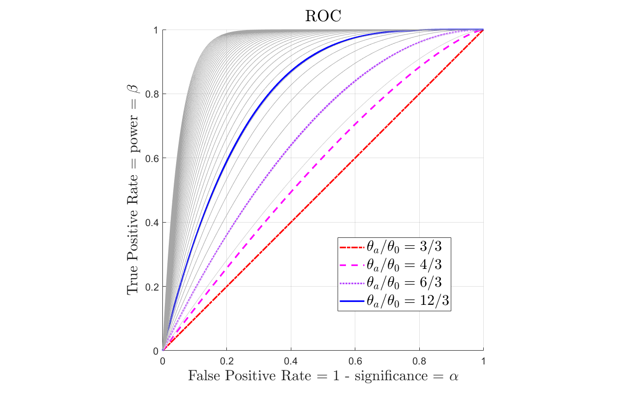
For general \(\theta_0, \theta_a\), the power is \(1 - (1 - \alpha)^{\theta_a/\theta_0}\). Sketch the power as a function of \(\alpha\) for \(\theta_0 = 3\), \(\theta_a = 4\) and for \(\theta_0 = 3\), \(\theta_a = 6\). This curve is the “receiver operator characteristic” (ROC). How does the ROC change if \(\theta_a \gg \theta_0\)? What if \(\theta_a \approx \theta_0\)?
Answer
The ROC curves should all start at 0, end at 1, should be monotonically decreasing, and should be concave down. They should increase monotonically for any fixed \(\alpha\) as \(\theta_a/\theta_0\) increases.
Try sketching by inspecting the function rather than jumping straight to a plotting tool — that skill matters on exams.
Check key properties first. Evaluate the power when \(\alpha = 0\) (power \(= 0\)) and \(\alpha = 1\) (power \(= 1\)). Is the function increasing or decreasing in \(\alpha\)? (increasing) Is it convex or concave? (concave).
No calculus needed! It is increasing since \((1 - \alpha)\) is decreasing as \(\alpha\) increases, so \((1 - \alpha)^p\) is decreasing for any positive power \(p\), and thus \(1 - (1 - \alpha)^p\) is increasing. It is concave since \((1 - \alpha)^p\) is convex for any \(p > 1\) (e.g. try \(p = 2\)), so \(1 - (1 - \alpha)^p\) is concave for any \(p > 1\). These are general properties of the ROC for well-designed tests — if you want extra confidence, you can compute the first and second derivatives.
In general, these ROC curves start at zero, end at one, are monotonically increasing, concave, are close to linear when \(\theta_a \approx \theta_0\), then converge towards the outer boundary of the ROC plot (power \(= 1\) for all \(\alpha \neq 0\)) as \(\theta_a/\theta_0\) diverges. To see why, note that \(1 - \alpha \in (0,1)\), so the larger the ratio \(\theta_a/\theta_0\), the smaller \((1 - \alpha)^{\theta_a/\theta_0}\), and thus the larger the power.
So the larger the ratio between \(\theta_a\) and \(\theta_0\), the more powerful the test for a fixed significance. As the ratio diverges, the power approaches one — the decision task gets easier because the distributions of \(x\) under the null and alternative become more distinct.
In contrast, if \(\theta_a \approx \theta_0\), then the power is approximately \(1 - (1 - \alpha) = \alpha\), which is the ROC for a uniform random test. If \(\theta_a = \theta_0\), the null and alternative are identical, so they are indistinguishable no matter what is observed — any decision rule between them is a coin toss.
2.2 ROC Curves
An ROC curve plots \(\text{TPR}\) against \(\text{FPR}\) as the decision threshold varies.
Definitions \[ \text{TPR} = \frac{\text{TP}}{\text{TP} + \text{FN}}, \qquad \text{FPR} = \frac{\text{FP}}{\text{FP} + \text{TN}}. \]
Building an ROC from finite data
- Compute the score \(s\) for each example.
- Consider thresholds between consecutive score values (plus \(\pm\infty\)).
- At each threshold, count TP/FP/FN/TN and plot \((\text{FPR}, \text{TPR})\).
Mixing / randomization
- Pure thresholds give the discrete ROC points (and the step-like curve connecting them).
- Randomly choosing between two thresholds with probabilities \(p\) and \(1-p\) yields any convex combination of their \((\text{FPR}, \text{TPR})\) points.
- Achievable pairs are exactly the convex hull of the pure-ROC points.
- Well-designed classifiers have a concave-down ROC; if yours dips inward, mixing can improve it.
- Points with \(\text{TPR} < \text{FPR}\) (below the diagonal) are typically not useful — you could flip labels / randomize to do at least as well as chance.
As you work through this question, focus on: 1. Manually plotting an ROC curve from data, and thinking about which thresholds achieve a given point (and which cannot) — you’ll implement related ideas in lab. 2. Understanding the shape of the achievable region (why can’t you land below the \(y = x\) line?). 3. Connecting this toy example to generic classifiers.
In lecture we discussed ROC curves, or “receiver operating characteristic” curves. ROC curves plot the true positive rate (TPR) and false positive rates (FPR) for a binary classifier at different decision thresholds. Recall that the TPR and FPR are defined as: \[\text{TPR} = \frac{\text{TP}}{\text{FN} + \text{TP}}, \quad \text{FPR} = \frac{\text{FP}}{\text{TN} + \text{FP}},\] where TP, TN, FP, and FN correspond to the entries of the 2 \(\times\) 2 table for binary decisions.
In this exercise, we will examine the ROC curve for a toy dataset. Let \(Y\) denote the true label for each example. Let \(X_1, X_2\) be observed features for each example. Suppose we adopt a test statistic \(s(X_1, X_2) = 3X_1 + 2X_2 + 1\), and decide whether to classify each example as a 0 or a 1 by comparing \(s(X_1,X_2)\) to a threshold \(s_*\).
| \(Y\) | \(s(X_1, X_2)\) | \(X_1\) | \(X_2\) |
|---|---|---|---|
| 0 | -1 | -1 | 0.5 |
| 1 | -0.5 | -1 | 0.75 |
| 0 | 0 | -1 | 1 |
| 1 | 1 | 0.2 | -0.3 |
| 1 | 0.25 | -0.25 | 0 |
| 0 | 0.25 | -0.05 | -0.3 |
Example dataset
2.2.1 (a)
Drawing a ROC Curve
Plot the ROC curve for the model \(f(X_1, X_2)\) with respect to the label \(Y\).
Answer
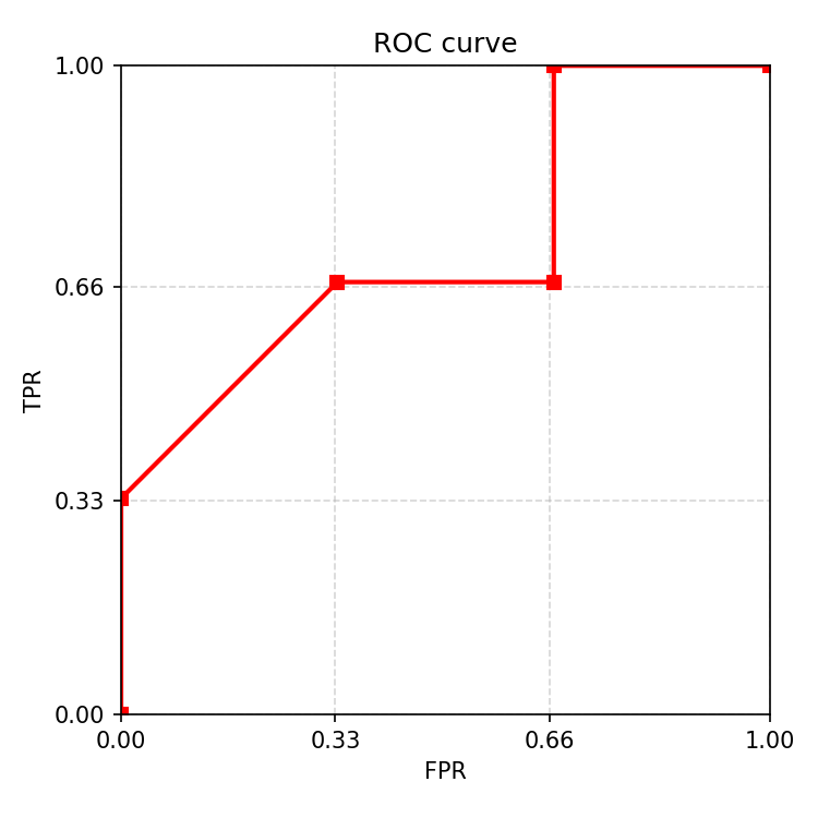
At a given decision threshold \(s_*\), if \(s(X_1, X_2) > s_*\), then the decision is a positive classification, and if \(s(X_1, X_2) \leq s_*\), then the decision is a negative classification. Since the model \(s(X_1, X_2)\) only takes five different values on this dataset, only six different ranges of decision thresholds produce distinct true and false positive rates.
\(s_* \in (-\infty,-1)\): \(\text{TPR} = 1\), \(\text{FPR} = 1\)
\(s_* \in [-1,-0.5)\): \(\text{TPR} = 1\), \(\text{FPR} = \frac{2}{3}\)
\(s_* \in [-0.5, 0)\): \(\text{TPR} = \frac{2}{3}\), \(\text{FPR} = \frac{2}{3}\)
\(s_* \in [0,0.25)\): \(\text{TPR} = \frac{2}{3}\), \(\text{FPR} = \frac{1}{3}\)
\(s_* \in [0.25, 1)\): \(\text{TPR} = \frac{1}{3}\), \(\text{FPR} = 0\)
\(s_* \in [1, \infty)\): \(\text{TPR} = 0\), \(\text{FPR} = 0\)
Plotting each (FPR, TPR) combination as a point on a plot results in the following ROC curve:
First, we identify what possible thresholds we can have. Seen from Table 1, \(s(X_1, X_2)\) takes on 5 different values – -1, -0.5, 0, 0.25, and 1. Using these 5 values we can produce 6 decision thresholds. Note that it is possible to do less thresholds but it will not be as inclusive; 6 is the maximum we can do given the number of data points.
Then, we can find the FPR and TPR at each threshold using the formulas defined at the start of the problem. Let’s use threshold \(s_*= 0.25\) as an example In this case, we classify examples with \(s(X_1, X_2) > 0.25\) as positive (1), and \(s(X_1, X_2) \leq 0.25\) as negative (0).
| Y (Actual) | \(s(X_1, X_2)\) | Predicted (if \(s_* = 0.25\)) | Outcome |
|---|---|---|---|
| 0 | -1 | 0 (negative) | TN |
| 1 | -0.5 | 0 (negative) | FN |
| 0 | 0 | 0 (negative) | TN |
| 1 | 1 | 1 (positive) | TP |
| 1 | 0.25 | 0 (negative) | FN |
| 0 | 0.25 | 0 (negative) | TN |
Classification results for \(s_* = 0.25\)
In total, we get 1 TP, 2 FNs, 0 FPs, and 3 TNs. Inputting these values into the formula for TPR and FPR, we get as follows: \[\text{TPR} = \frac{\text{TP}}{\text{FN} + \text{TP}} = \frac{1}{1 + 2} = \frac{1}{3}\] \[\text{FPR} = \frac{\text{FP}}{\text{TN} + \text{FP}} = \frac{0}{0 + 3} = 0\]
2.2.2 (b)
Mixing Decision Criteria
You should notice that your ROC curve looks a bit odd. It has a step between FPR 0.33 and 0.66. Can we do better here? Propose a mixed test where we select two thresholds \(s_*\) and \(s'_*\), and, when we apply the test, pick between the two tests randomly.
Answer
Yes! In general, we can produce a test with any pair of \((\text{FPR}, \text{TPR}) = (\alpha,\beta)\) if the pair \((\alpha, \beta)\) can be produced as some weighted average of points on the original ROC curve. That is, we can produce any FPR, TPR pair in the convex hull of the ROC curve corresponding to pure tests. To draw a convex hull, find the smallest convex polygon containing the original curve, or, draw straight-lines between all corners/vertices in the curve, and keep the outermost boundary.
We will accomplish this by mixing tests. This process also explains why the ROC is usually concave down, and is concave down if optimal. If the ROC is not concave down, then it could be improved by mixing tests.
In particular, pick \(s_* \in [0,0.25)\) and \(s'_* = [-0.5,0)\), then mix the tests by choosing the first threshold with probabiliy \(p\), and the second with probability \(p' = 1 - p\) for some \(p \in (0,1)\). The result is a test whose ROC lies on the line segment connecting the “corners” of the original ROC plot (the points \((1/3,2/3)\) and \((2/3,1)\)). The line segment lies above the original ROC.
Try a concrete example. Pick the suggested \(s_*\) and \(s_*'\), and set \(p = 1/2\). Compute the FPR and TPR. Then repeat with \(p = 3/4\) and look for the pattern. In general, \[ (\alpha(p),\beta(p)) = p(\alpha,\beta) + (1 - p) (\alpha',\beta'), \] which you can derive by partitioning outcomes into: (1) draw a threshold at random, then (2) apply the corresponding test.
Being able to draw the convex hull is especially useful for the next part. Looking back at problem 1, ROC plots for well-designed tests usually curve downwards — they are concave because they are the upper boundary of a convex achievable region of (FPR, TPR) pairs.
2.2.3 (c)
More Mixing
Is it possible to choose two decision thresholds \(s_*, s_*'\) and probabilities of using each decision threshold such that the expected false positive rate is \(\frac{2}{3}\), and the expected true positive rate is \(\frac{1}{3}\)?
Answer
No single threshold or combination of two thresholds can achieve a false positive rate of \(\frac{2}{3}\) without also increasing the true positive rate up to \(\frac{2}{3}\) (try it!).
By choosing probabilities for using each decision threshold \(s_*\) and \(s_*'\), the expected TPR and FPR are a convex combination of the TPRs and FPRs of \(s_*\) and \(s_*'\) individually. Specifically, any (FPR, TPR) pair that is not a convex combination of the (FPR, TPR) pairs for single thresholds (plotted on the ROC curve) cannot be achieved by choosing two decision thresholds probabilistically.
Using the convex hull idea from the previous part, note that the lower boundary is the line from \((0,0)\) to \((1,1)\). The convex hull never includes a point with \(\text{TPR} < \text{FPR}\).