7 Data 102 Discussion 07: Generalized Linear Models
7.0.1 Contact Information
| Name | Wesley Zheng |
| Pronouns | He/him/his |
| wzheng0302@berkeley.edu | |
| Discussion | Wednesdays, 11–12 PM @ Wheeler 224 |
| Office Hours | Tuesdays, 9–10 AM & 11-12 PM @ Gateway B1040 |
Contact me by email at ease — I typically respond within a day or so!
7.1 Poisson Regression
Suppose you’re curious about the average number of chocolate cupcakes Cupcakin’ Bake Shop sells per minute on a given day. This number depends on the number of people who pass by the bakery on that day.
For a given day \(i\), let \(Y_{ij}\) denote the number of cupcakes sold during minute \(j\) of day \(i\), let \(X_i\) denote the number of people who pass the bakery on day \(i\), and let \(\lambda(X_i)\) denote the average number of cupcakes sold per hour on day \(i\).
7.1.1 (a)
Choosing a Distribution
Write down a plausible distribution for \(Y_{ij} \mid X_i\).
Hint: There are multiple possible answers.
Answer
A reasonable choice is the Poisson distribution: \[ Y_{ij} \mid X_i \sim \operatorname{Poisson}\left(\frac{\lambda(X_i)}{60}\right). \]
The Poisson distribution is commonly used to model counts of events occurring within a fixed time interval. Since \(\lambda(X_i)\) represents the expected number of cupcakes sold per hour, dividing by \(60\) gives the expected number sold per minute.
7.1.2 (b)
Identifying the Link Function
Suppose you learn that \[ \lambda(X_i) = e^{\beta_0 + \beta_1 X_i} \] for some parameters \(\beta_0\) and \(\beta_1\).
What is the link function \(g\) such that \[ \lambda(X_i) = g^{-1}(\beta_0 + \beta_1 X_i)? \]
Answer
The link function is \[ g(z) = \log(z). \]
Taking the logarithm of both sides gives \[ \log(\lambda(X_i)) = \beta_0 + \beta_1 X_i. \] Therefore, the link function is the natural logarithm, while the inverse link function is the exponential function.
7.1.3 (c)
Interpreting the Coefficient
Suppose the number of people passing by the bakery increases by one, from \(X_i\) to \(X_i + 1\).
By what factor does the expected number of cupcakes sold per hour change? Express your answer in terms of \(\beta_1\).
Answer
The ratio of expected sales rates is \[ \begin{align*} \frac{\lambda(X_i+1)}{\lambda(X_i)} &= \frac{e^{\beta_0+\beta_1(X_i+1)}}{e^{\beta_0+\beta_1 X_i}} \\ &= e^{\beta_1}. \end{align*} \]
Therefore, increasing \(X_i\) by one multiplies the expected number of cupcakes sold per hour by \(e^{\beta_1}\).
Unlike ordinary linear regression, where coefficients represent additive changes in the expected response, coefficients in Poisson regression with a log link represent multiplicative changes.
For example, if \(\beta_1 = \log(2)\), then each additional person passing by doubles the expected sales rate.
7.1.4 (d)
Deriving the Likelihood
Suppose we observe cupcake sales over \(n\) days. For each day \(i\), we observe \(m_i\) minutes of sales and the number of people \(X_i\) who pass by the bakery.
Using the Poisson regression model from Parts (a) and (b), write down the conditional probability \(P(Y_{ij}=y_{ij}\mid X_i)\). Then, assuming conditional independence, derive the likelihood function \(L(\beta_0,\beta_1)\) for the entire dataset.
Answer
From Parts (a) and (b), we have \[ Y_{ij}\mid X_i \sim \operatorname{Poisson}\left(\frac{e^{\beta_0+\beta_1 X_i}}{60}\right). \]
Recall that the probability of observing \(Y=y\) under a Poisson distribution with mean \(\mu\) is \[ P(Y=y)=\frac{\mu^y e^{-\mu}}{y!}. \]
Substituting the mean from our model gives \[ P(Y_{ij}=y_{ij}\mid X_i) = \frac{ \left(\frac{e^{\beta_0+\beta_1 X_i}}{60}\right)^{y_{ij}} e^{-e^{\beta_0+\beta_1 X_i}/60} }{y_{ij}!}. \]
Since the observations are conditionally independent, the likelihood is \[ L(\beta_0,\beta_1) = \prod_{i=1}^{n}\prod_{j=1}^{m_i} \frac{ \left(\frac{e^{\beta_0+\beta_1 X_i}}{60}\right)^{y_{ij}} e^{-e^{\beta_0+\beta_1 X_i}/60} }{y_{ij}!}. \]
The Poisson mean must match the time interval used for the response. Here, \(\lambda(X_i)\) is an hourly rate, while \(Y_{ij}\) counts sales in one minute, so the minute-level mean is \(\lambda(X_i)/60\). Under conditional independence, multiply the conditional probabilities across all days and minutes to obtain the likelihood.
7.2 Interpreting the Logistic Regression Model
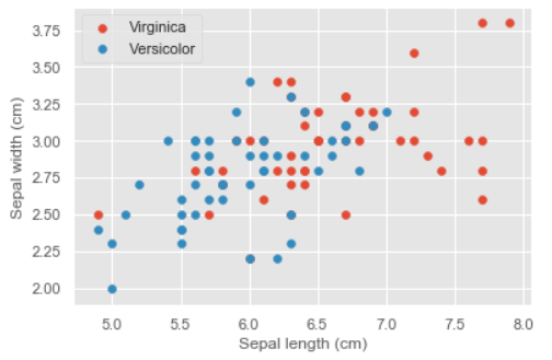
In this problem, we fit a logistic regression model on a subset of the famous iris dataset. We have 100 samples of iris flowers, and measure their sepal length, sepal width, petal length and petal width (sepals are the small, green growths at the base of a flower). The response labels are whether they belong to the Virginica species (1) or the Versicolor species (0).
Let’s say we first fit a Logistic regression model to predict the iris species, using only the sepal features. Then, our data is represented in the following plot:
7.2.1 (a)
Reformulating Logistic Regression
From lecture, we have seen that Logistic Regression applies the sigmoid inverse link function to map a linear predictor \(x_i^T \beta\) to probabilities in the following way: \[ \sigma(x_i^T \beta) = \frac{1}{1 + e^{-x_i^T \beta}} = p \in (0, 1) \] where \(p\) is the probability of the \(i\)-th data point belonging to class \(1\). Reformulate Logistic Regression in terms of the \(logit\) link function.
Answer
Recall that the role of a link function is to transform its input into a linear predictor, \(x_i^T \beta\). We can solve for \(x_i^T \beta\) using the following steps: \[ \begin{align*} \frac{1}{1 + e^{-x_i^T \beta}} &= p \\ 1 + e^{-x_i^T \beta} &= \frac{1}{p} \\ e^{-x_i^T \beta} &= \frac{1 - p}{p} \\ -x_i^T \beta &= \log\left(\frac{1 - p}{p}\right) \\ x_i^T \beta &= \log\left(\frac{p}{1 - p}\right) \end{align*} \]
The term inside the \(\log\) has a special name—the odds ratio. This ratio takes on values in \((0, \infty)\), where values in \((0, 1)\) indicate that \(1 - p > p\), while values in \((1, \infty)\) indicate that \(p > 1 - p\).
7.2.2 (b)
Interpreting a coefficient of a Logistic model
Suppose after fitting the aforementioned logistic regression model, you observe the following output:
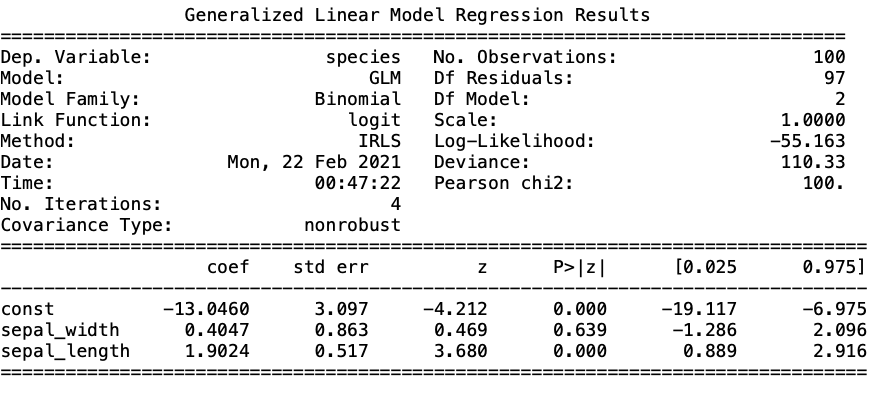
Assuming that the model is correct, use the derivation in Part (a) to write a one sentence interpretation for the logistic model with respect to sepal length. What happens to the interpretation if the model is misspecified?
Answer
Holding sepal width constant, every 1 cm increase in sepal length increases the log odds ratio of the iris belonging to Virginica (rather than Versicolor) by between 0.9 and 2.9. If the model is misspecified, then the interpretation is only valid with respect to the projected model.
Using the coefficients of constant, sepal width, and sepal length from the table, we can form the following equation: \[ \log\left(\frac{p}{1 - p}\right) = -13.05 + 0.40w + 1.90l \] where \(p\) = probability that \(X_i\) is Virginia. With this, we derive that a longer sepal length (represented by \(l\)) will lead to a higher probability that \(X_i\) is Virginia. In other words, a unit increase in sepal length corresponds to a ~1.90 increase in the log-odds of \(X_i\) being Virginica.
7.2.3 (c)
Deriving the Likelihood
Recall that \(Y_i=1\) if flower \(i\) belongs to the Virginica species and \(Y_i=0\) if it belongs to the Versicolor species. Let \(x_i=(1,w_i,l_i)^T\) denote the intercept, sepal width, and sepal length of flower \(i\).
Using the logistic regression model from Part (a), specify the conditional distribution of \(Y_i\mid x_i\) and derive the likelihood function \(L(\beta)\) for the 100 observations, assuming independence.
Answer
Since \(Y_i\) is binary, we model it using a Bernoulli distribution: \[ Y_i\mid x_i \sim \operatorname{Bernoulli}(p_i), \] where \[ p_i=\frac{1}{1+e^{-x_i^T\beta}}. \]
The probability of observing \(Y_i=y_i\) is \[ P(Y_i=y_i\mid x_i) = p_i^{y_i}(1-p_i)^{1-y_i}. \]
Since the observations are independent, the likelihood is \[ L(\beta) = \prod_{i=1}^{100} p_i^{y_i}(1-p_i)^{1-y_i}. \]
Substituting the expression for \(p_i\), we obtain \[ L(\beta) = \prod_{i=1}^{100} \left(\frac{1}{1+e^{-x_i^T\beta}}\right)^{y_i} \left(\frac{1}{1+e^{x_i^T\beta}}\right)^{1-y_i}. \]
The sigmoid function gives the Bernoulli success probability \(p_i\). Each observation contributes \(p_i^{y_i}(1-p_i)^{1-y_i}\) to the likelihood; independence lets us multiply these contributions across all 100 observations.