3 Data 102 Discussion 03: Multiple Hypothesis Testing
3.0.1 Contact Information
| Name | Wesley Zheng |
| Pronouns | He/him/his |
| wzheng0302@berkeley.edu | |
| Discussion | Wednesdays, 11–12 PM @ Wheeler 224 |
| Office Hours | Tuesdays, 9–10 AM & 11-12 PM @ Gateway B1040 |
Contact me by email at ease — I typically respond within a day or so!
3.1 Hypothesis Testing and Classification
Rows of the \(2\times 2\) table are reality; columns are the decision.
Row-wise rates (condition on reality): \[ \text{FPR} = \frac{\text{FP}}{\text{FP}+\text{TN}}, \quad \text{TPR} = \frac{\text{TP}}{\text{TP}+\text{FN}}, \quad \text{FNR} = \frac{\text{FN}}{\text{TP}+\text{FN}} = 1 - \text{TPR}. \]
Column-wise rates (condition on the decision): \[ \text{FDP} = \frac{\text{FP}}{\text{FP}+\text{TP}} = \mathbb{P}(R=0 \mid D=1), \qquad \text{TDR} = 1 - \text{FDP} = \mathbb{P}(R=1 \mid D=1). \]
\(p\)-values (under a continuous null):
- A small \(p\)-value is evidence against the null (favoring the alternative).
- Under the null, \(p\)-values are Uniform\([0,1]\), so \(\mathbb{P}(p \le \alpha \mid H_0) = \alpha\).
Bayes for disease testing: with prevalence \(\pi\), sensitivity \(\text{TPR}\), and FPR, \[ \mathbb{P}(\text{disease} \mid \text{positive}) = \frac{\text{TPR}\,\pi}{\text{TPR}\,\pi + \text{FPR}\,(1-\pi)}. \]
In this question, we review classification metrics, \(p\)-values, conditional probabilities, and hypothesis testing.
3.1.1 (a)
In the following table, rows represent reality and columns represent the decision:
| 0 | 1 | |
|---|---|---|
| 0 | 4 | 7 |
| 1 | 3 | 2 |
Compute the following:
3.1.1.1 (i)
FPR (false positive rate)
Answer
\(\text{FPR} = \frac{\text{FP}}{\text{FP}+\text{TN}}\), or \[ \frac{7}{4+7} = \frac{7}{11}. \]
3.1.1.2 (ii)
TPR (true positive rate)
Answer
\(\text{TPR} = \frac{\text{TP}}{\text{TP}+\text{FN}}\), or \[ \frac{2}{2+3} = \frac{2}{5}. \]
3.1.1.3 (iii)
FNR (false negative rate)
Answer
\(\text{FNR} = \frac{\text{FN}}{\text{TP}+\text{FN}}\), or \[ \frac{3}{2+3} = \frac{3}{5}. \]
3.1.1.4 (iv)
FDP (false discovery proportion)
Answer
Unlike the previous three, this is a column-wise rather than row-wise rate. We have \[ \text{FDP} = \frac{\text{FP}}{\text{FP}+\text{TP}} = \frac{7}{7+2} = \frac{7}{9}. \]
3.1.1.5 (v)
Is the classifier represented by this table a good or a bad classifier? Why?
Answer
It is a bad classifier, because flipping the decision (all 0s become 1s and vice versa) would improve every single metric. In other words, it is worse than chance.
3.1.2 (b)
Answer the following conceptual questions about \(p\)-values:
3.1.2.1 (i)
Circle the correct bold-faced word: Small \(p\)-values give evidence that the null/alternative hypothesis is true.
Answer
Alternative.
3.1.2.2 (ii)
Complete the statement: Under the null hypothesis, the distribution of \(p\)-values is ____.
Answer
Uniform \([0,1]\).
3.1.2.3 (iii)
If the null hypothesis is true, what is the probability of obtaining a \(p\)-value that is less than or equal to \(0.01\)?
Answer
\(0.01\).
3.1.3 (c)
Consider a test for a disease, where the test has a false positive rate of \(1\%\) and a true positive rate of \(80\%\).
3.1.3.1 (i)
Suppose the proportion of people that have the disease is \(5\%\). Conditional on a positive test, how likely is a person to actually have the disease?
Answer
Algebraically, we can apply Bayes’ rule. But the easiest way to visualize this is to imagine \(100\) people, \(5\) of whom have the disease and \(95\) of whom do not. If all of them take the test, \(4\) of the people with the disease will test positive and \(0.95\) of those who do not have the disease will test positive. Therefore, \[ \mathbb{P}(\text{disease} \mid \text{positive}) = \frac{4}{4+0.95} = \frac{80}{99}. \]
3.1.3.2 (ii)
What is the name of the conditional probability in the previous question?
Answer
True discovery rate.
3.1.3.3 (iii)
Suppose instead that the proportion of people with the disease is \(0.1\%\). Now how likely is a person to have the disease, conditional on a positive test?
Answer
We can apply the same visualization as before. Imagine \(1000\) people, \(1\) with the disease and \(999\) without. Then in expectation, \(0.8\) of the people with the disease test positive, and \(9.99\) without the disease test positive. Therefore, \[ \mathbb{P}(\text{disease} \mid \text{positive}) = \frac{0.8}{0.8+9.99} = \frac{80}{1079}. \]
3.1.4 (d)
For a real-valued random variable \(X\), consider the following two hypotheses: \[ H_0: X \sim \operatorname{Uniform}([0,1]), \qquad H_1: X \sim \operatorname{Uniform}([0.5,1.5]). \]
We would like a test with a false positive rate of at most \(0.05\). What is the best possible true positive rate?
Answer
The best we can do is reject the null when \(X > 0.95\), which has a false positive rate of exactly \(0.05\). Then under \(H_1\), we correctly output \(1\) when \[ X \in [0.95,1.5] \] and incorrectly output \(0\) when \[ X \in [0.5,0.95]. \] Therefore, the best possible true positive rate is \[ 0.55. \]
Interestingly, Neyman–Pearson does not apply in the usual way here, because the likelihood ratio is not a continuous function of \(X\) (the two densities have overlapping support with flat pieces, so the LR takes only a few discrete values).
3.2 Multiple Hypothesis Testing with the Benjamini–Hochberg Procedure
Goal: control the false discovery rate (FDR) at level \(\alpha\) when testing many hypotheses at once.
Algorithm
- Input: FDR level \(\alpha\), and \(n\) \(p\)-values \(P_1,\ldots,P_n\).
- Sort them: \(P_{(1)} \le P_{(2)} \le \cdots \le P_{(n)}\).
- Find \[ K = \max\left\{i\in\{1,\ldots,n\}: P_{(i)} \le \frac{\alpha}{n}\, i\right\} \] (if no such \(i\) exists, set \(K=0\)).
- Reject the nulls corresponding to \(P_{(1)},\ldots,P_{(K)}\).
BH line: compare the \(k\)-th ordered \(p\)-value to \(y(k) = k\cdot\alpha/n\).
Important subtlety: \(K\) is the largest index with \(P_{(K)} \le y(K)\). You do not stop at the first crossing; a later \(p\)-value can pull the threshold up and cause earlier hypotheses to be rejected even if some intermediate \(P_{(k)} > y(k)\).
In this question we analyze the properties of the Benjamini–Hochberg (BH) procedure. Recall the steps of the procedure:
- Input: FDR level \(\alpha\), set of \(n\) \(p\)-values \(P_1,\ldots,P_n\).
- Sort the \(p\)-values in non-decreasing order \(P_{(1)}\le P_{(2)}\le \cdots \le P_{(n)}\).
- Find \(K = \max\left\{i\in\{1,\ldots,n\}: P_{(i)} \le \frac{\alpha}{n} i\right\}\).
- Reject the null hypotheses (declare discoveries) corresponding to \(P_{(1)},\ldots, P_{(K)}\).
3.2.1 (a)
We have 10 \(p\)-values for multiple hypothesis testing: 0.001, 0.003, 0.012, 0.015, 0.08, 0.09, 0.1, 0.14, 0.16, 0.28. Suppose we would like to control the FDR at the level \(0.05\). How many tests does the BH procedure reject?
Answer
By first sorting the \(p\)-values and comparing the \(k\)-th \(p\)-value with \(k \cdot \alpha /n = 0.005k\), we will see that the largest \(k\) such that its \(p\)-value is smaller than \(0.005k\) is \(k=4\). So 4 tests will be rejected.
First, ensure the \(p\)-values are sorted in non-decreasing order: 0.001, 0.003, 0.012, 0.015, 0.08, 0.09, 0.1, 0.14, 0.16, 0.28. Let \(p_k\) be the \(k\)th ordered \(p\)-value.
Next, form the BH line \(y(k)\), which is what we compare \(p\)-values against: \[ y(k) = k\frac{\alpha}{n} = k\frac{0.05}{10} = 0.005 k, \] where \(\alpha = 0.05\) and \(n = 10\).
Going one by one down the sorted list:
- First \(p\)-value 0.001, \(y=1(0.005) = 0.005\). \(p\)-value is smaller.
- Second \(p\)-value 0.003, \(y=2(0.005) = 0.010\). \(p\)-value is smaller.
- Third \(p\)-value 0.012, \(y=3(0.005) = 0.015\). \(p\)-value is smaller.
- Fourth \(p\)-value 0.015, \(y=4(0.005) = 0.020\). \(p\)-value is smaller.
- Fifth \(p\)-value 0.080, \(y=5(0.005) = 0.025\). \(p\)-value is bigger — stop checking further for a larger valid \(k\).
The largest \(k\) with \(p_k \le y(k)\) is \(k=4\), so the threshold is \(p_4 = 0.015\). Reject all tests with \(p \le 0.015\): 4 discoveries.
Note: The threshold is the largest \(p\)-value beneath \(y_k\). That is not the same as stopping at the first crossing of \(y_k\). In general, BH could reject some index \(k\) with \(p_k > y_k\) if a later index \(k' > k\) still satisfies \(p_{k'} \le y_{k'}\).
3.2.2 (b)
Suppose \(P_1 = P_2 = \dots = P_n=\alpha\), and we run BH under level \(\alpha\) on these \(p\)-values. How many discoveries does BH make? Explain.
Answer
It makes \(n\) discoveries, because the highest \(p\)-value (equal to \(\alpha\)) is less than or equal to \(\frac{\alpha}{n}n = \alpha\).
Plot the BH critical values against \(k\) — this is the BH guideline:
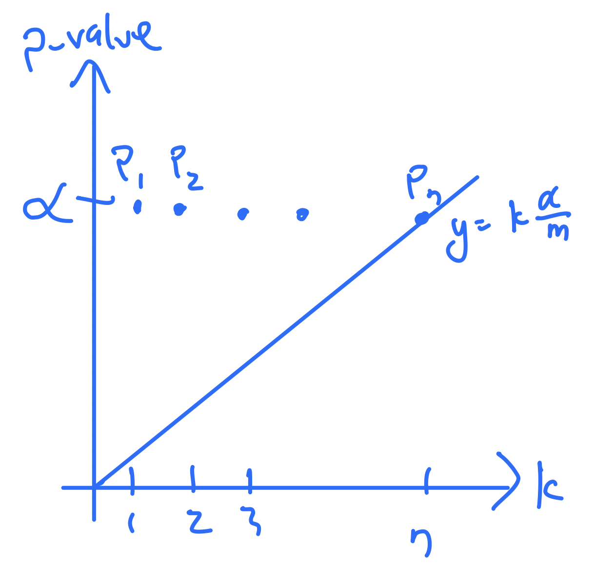
Comparing each \(p\)-value against the BH guideline, all values lie above the guideline except the last one (equal to \(\alpha\)). Since that last point is still on/under the line, the threshold is \(\alpha\), and every \(p\)-value is at or below it — so BH rejects all \(n\) hypotheses.
3.2.3 (c)
Suppose \(P_1 = P_2 = \dots = P_{n-1}=\alpha\), \(P_n = \alpha + 0.001\alpha\), and we run BH under level \(\alpha\) on these \(p\)-values. How many discoveries does BH make? Explain.
Answer
It makes 0 discoveries, because no \(p\)-value is under the corresponding threshold \(\frac{\alpha}{n}k\).
If we draw the BH line, all the \(p\)-values sit above it, so no discoveries are made:
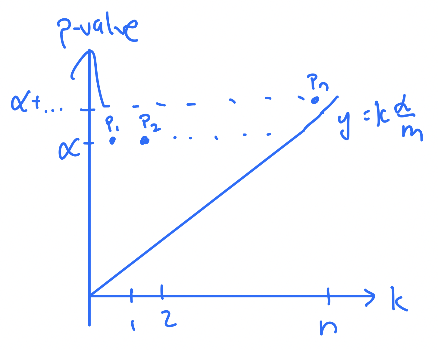
If this is hard to see visually, check one-by-one: Is \(P_1 \le \frac{\alpha}{n}\)? How about \(P_2 \le 2\frac{\alpha}{n}\)? And so on — none satisfy the inequality.
3.2.4 (d)
Suppose we run BH on \(\{P_1,\ldots,P_n\}\), and we make \(R<n\) discoveries. Now suppose we add an extra \(p\)-value equal to 0 to this set. Now we run BH on \(\{P_1,\ldots,P_n,0\}\) and get a new number of rejections \(R'\). Which of the following are possible: \(R'>R\), \(R'=R\), \(R'<R\)? If multiple are possible, list all that are possible. Explain why.
Answer
The new \(p\)-value 0 is now the smallest one in the sequence. Therefore, if some given \(p\)-value was compared to \(\frac{\alpha}{n}k\) before adding the extra \(p\)-value, now it’s compared to \(\frac{\alpha}{n+1}(k+1)\). Since \(\frac{\alpha}{n+1}(k+1)>\frac{\alpha}{n}k\), it is now strictly easier to discover. Moreover, the new \(p\)-value 0 will definitely be discovered, so \(R'>R\) is the only possibility.
How the BH guideline changes:
- \(n\) becomes \(n+1\).
- Every old \(p\)-value shifts one index to the right (the new 0 is first), so its comparison index goes from \(k\) to \(k+1\).
The new critical value satisfies \(\frac{\alpha}{n+1}(k+1) > \frac{\alpha}{n}k\), so the bar is higher for each shifted \(p\)-value. Combined with definitely rejecting the new \(p=0\), we must have \(R'>R\).
3.2.5 (e)
Suppose we run BH on \(P_1,\ldots,P_n\), and we make \(R<n\) discoveries. Now suppose we add an extra \(p\)-value equal to the maximum \(p\)-value in this set; denote that \(p\)-value \(P_{\max}\). Now we run BH on \(P_1,\ldots,P_n,P_{\max}\) and get a new number of rejections \(R'\). Which of the following are possible: \(R'>R\), \(R'=R\), \(R<R\)?
Answer
The new \(p\)-value will be the largest one in the sequence. Therefore, if any given \(p\)-value was compared to level \(\frac{\alpha}{n}k\) before adding the extra \(p\)-value, now it will be compared to \(\frac{\alpha}{n+1}k<\frac{\alpha}{n}k\). It is thus impossible to have \(R'>R\); the other two options are possible.
Again \(n\) becomes \(n+1\), but now \(P_{\max}\) is still the maximum, so the relative order of the original \(p\)-values is unchanged and their indices \(k\) stay the same.
The BH critical value becomes \(\frac{\alpha}{n+1}k < \frac{\alpha}{n}k\), which makes discoveries harder. So \(R'>R\) is impossible, while \(R'=R\) and \(R'<R\) remain possible.