6 Data 102 Discussion 06: Graphical Models & Gibbs Sampling
6.0.1 Contact Information
| Name | Wesley Zheng |
| Pronouns | He/him/his |
| wzheng0302@berkeley.edu | |
| Discussion | Wednesdays, 11–12 PM @ Wheeler 224 |
| Office Hours | Tuesdays, 9–10 AM & 11-12 PM @ Gateway B1040 |
Contact me by email at ease — I typically respond within a day or so!
6.1 Graphical Models
A graphical model (Bayes net) is a DAG where each node is a random variable and an arrow \(A \to B\) means “\(A\) directly influences \(B\).” The graph tells you how the joint distribution factors: \[ p(x_1, \ldots, x_n) = \prod_{i} p(x_i \mid \text{parents}(x_i)). \]
If you took CS 188, my notes there practice exactly these skills: factoring the joint (Disc 06, Q1(a) and Bayes Nets: Representation) and drawing a net from a word description (Disc 06, Q2(e)). The tricks that carry over:
Drawing a model from a story. For each variable, ask “what directly affects this?” and draw arrows from those variables into it. A missing arrow is a modeling assumption: if nothing connects two root nodes, you are assuming they are independent.
Reading independence off the graph. Every path between two variables is built from three patterns:
- Chain \(w \to y \to z\): observing the middle node \(y\) blocks the path.
- Common cause \(w \leftarrow y \to z\): observing \(y\) blocks the path.
- Common effect \(w \to y \leftarrow x\): the path is blocked unless \(y\) (or a descendant of \(y\)) is observed. Observing the common effect makes its causes dependent (“explaining away”).
d-separation turns these patterns into a test. To check whether \(A \perp \! \! \! \perp B \mid \text{evidence}\), look at every path between \(A\) and \(B\):
- A path is blocked if at least one pattern on it is blocked (an observed chain or common-cause middle node, or a common-effect middle node with neither it nor any descendant observed).
- A path is active if every pattern on it lets information through.
If every path is blocked, \(A\) and \(B\) are d-separated given the evidence, and the graph guarantees \(A \perp \! \! \! \perp B \mid \text{evidence}\). If even one path is active, they are d-connected, and the graph no longer guarantees independence, so they can be dependent. (The specific numbers in the tables could still happen to make them independent, but you can’t conclude that from the graph alone.)
Two shortcuts that follow from this: a node is independent of its non-descendants given its parents, and a node is independent of everything else given its Markov blanket (parents, children, and children’s other parents).
The CS 188 material for this:
- The CS 188 textbook section on d-separation explains causal chains, common causes, common effects, and how to check paths in larger graphs.
- The two shortcuts (independent of non-descendants given parents, and independent of everything given the Markov blanket) are the Bayesian Network Representation review in Disc 07.
- The Disc 06, Q2(c) checklist (“mark all that are guaranteed to be true”) is practice applying the three patterns to a larger net. For example, \(D \perp \! \! \! \perp E\) holds because \(D \to F \leftarrow E\) is a common effect with \(F\) unobserved.
- Disc 06, Q1(c) reads \(A \perp \! \! \! \perp B\) off the graph using d-separation, which is the name for these path-blocking rules.
In lecture, we were introduced to Graphical Models, which are flexible diagrams to express the relationships between random variables. An important special case of graphical models are Bayesian hierarchical models, which generally may look like the figure below:
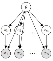
In a Bayesian hierarchical model, observations are independent given the latent variables, and each observed variable depends only on its corresponding latent variable and the hyperparameters. As a result, Bayesian hierarchical models are always depicted as directed acyclic graphs (DAGs).
In the following subparts, we will create our own graphical model and explore its properties.
6.1.1 (a)
Formulating a Graphical Model
Suppose you are a farmer who wants to model the upcoming crop harvest. You are interested in the following variables:
- \(w\) is the amount of pesticide used
- \(x\) is the amount of total rainfall for the season
- \(y\) is the number of bugs found in the field
- \(z\) is the total crop yield
Draw a graphical model to illustrate the relationships between these variables.
Answer
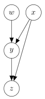
First, we can observe that there isn’t really any relationship between the amount of pesticide use and total rainfall, so we can safely assume that \(w\) and \(x\) are independent. Next, we observe that the bug count \(y\) is affected by both pesticide use \(w\) (i.e. more pesticides \(\rightarrow\) fewer bugs) and by rain \(x\). Lastly, rain has a direct effect on crop yield \(z\). Using this information, we can draw the following graphical model:
6.1.2 (b)
Identifying Independence and Conditional Independence
Consider the following graphical model:
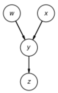
Which of the following statements are true about the graphical model above?
- \(x \perp \!\!\! \perp w\)
- \(w \perp \!\!\! \perp x \mid y\)
- \(w \perp \!\!\! \perp z \mid y\)
Answer
Statement 1 is True.
We can see this algebraically by writing out the joint distribution:
\[ p(w, x, y, z) = p(w)p(x)p(y \mid w, x) p(z \mid y) \]
Since we’re only interested in the relationship between \(w\) and \(x\), we need to marginalize over \(z\) and \(y\). \[ \begin{align*} p(w, x) &= \sum_y \sum_z \left[p(w)p(x)p(y \mid w, x) p(z \mid y)\right] \\ &= p(w)p(x) \sum_y \sum_z \left[p(y \mid w, x) p(z \mid y)\right] \\ &= p(w)p(x) \sum_y p(y \mid w, x) \underbrace{\left[\sum_z p(z \mid y)\right]}_{=1} \\ &= p(w)p(x) \underbrace{\sum_y p(y \mid w, x)}_{=1} \\ &= p(w)p(x) \end{align*} \]
This is precisely the definition of independence, so we’re done. Intuitively, when we marginalize a node in a graphical model, parents of that node usually aren’t affected.
Statement 2 is False.
We can follow a similar computation above. From the definition of conditional probability, \(p(w, x \mid y) = \frac{p(w, x, y)}{p(y)}\). Since this is a distribution over \(w\) and \(x\), the denominator is a constant.
\[ \begin{align*} p(w, x \mid y) &\propto p(w, x, y) \\ &= \sum_z \left[p(w)p(x)p(y \mid w, x) p(z \mid y)\right] \\ &= p(w)p(x)p(y \mid w, x) \underbrace{\sum_z p(z \mid y)}_{=1} \end{align*} \]
At this point, we can see that the conditional distribution does not factor because of the term \(p(y \mid w, x)\), so we can conclude that conditioned on \(y\), \(w\) and \(x\) are not independent.
Statement 3 is True.
For Bayesian hierarchical models, we know that given a particular node was observed, the node’s parents are independent of its children. Therefore, since \(y\) was observed, parent node \(w\) is independent of child node \(z\).
\[ \begin{align*} p(w,z \mid y) &= \frac{p(w,z,y)}{p(y)} \\ &= \frac{p(w)\sum_x \left[p(y \mid w, x)p(x)\right]p(z \mid y)}{\sum_w \sum_x \left[p(y \mid w, x)p(x)p(w)\right]} \\ &= \frac{p(w)p(z \mid y)\sum_x \left[p(y \mid w, x)p(x)\right]}{\sum_x \left[p(y \mid w, x)p(x)\right]} \\ &= p(w)p(z \mid y) \end{align*} \]
If you took CS 188, this is the same Bayes net machinery from my notes there. Writing the joint as \(p(w)p(x)p(y \mid w, x)p(z \mid y)\) is the “each node given its parents” factorization we used to compute \(P(+g, +a, +b, +s)\) in CS 188 Discussion 06, Q1(a).
Statement 3 is also an instance of a rule from the Bayes net representation review in CS 188 Discussion 07: each node is conditionally independent of its non-descendants given its parents. Here \(z\)’s only parent is \(y\), and \(w\) is a non-descendant of \(z\), so \(w \perp \!\!\! \perp z \mid y\).
6.2 Gibbs Sampling for Gamma-Poisson model
Gibbs sampling draws from a joint posterior \(\mathbb{P}(\theta_1, \ldots, \theta_d \mid X)\) that is hard to sample directly by repeatedly sampling one variable at a time from its full conditional \(\mathbb{P}(\theta_i \mid X, \theta_{-i})\), always conditioning on the most recent values of everything else. The data (evidence) never change. After enough iterations, the samples come from the joint posterior.
If you took CS 188, my notes there cover the same algorithm on discrete Bayes nets: the Gibbs sampling review, the Markov blanket rule, and a practice question on which sample sequences Gibbs can produce. The tricks that carry over:
Shrink the conditioning set with the Markov blanket. A variable’s full conditional only depends on its Markov blanket: its parents, its children, and its children’s other parents. Read these off the graph first and drop every other variable from the conditioning.
Keep only the factors that contain the variable. Write the joint as a product of “each node given its parents.” The full conditional of \(\theta_i\) is proportional to the factors that mention \(\theta_i\): its own factor \(p(\theta_i \mid \text{parents})\) and one factor per child \(p(\text{child} \mid \ldots, \theta_i, \ldots)\). Everything else is a constant you can drop with \(\propto\).
Recognize the kernel. Combine powers and exponents of the variable and match a known family, the same way as with conjugate priors in Discussion 4. For example, \[ u^{a-1} e^{-bu} \;\Longrightarrow\; \text{Gamma}(a, b). \]
Turn the conditionals into an algorithm. Initialize every unknown, then loop: resample each unknown from its full conditional using the newest values of the others. Variables that are conditionally independent of each other given the rest (e.g., none of them is in another’s Markov blanket) can be resampled at the same time.
When the dimension of the parameters is large, sampling from the posterior over all the parameters \(\theta\) is often difficult. The main insight behind Gibbs sampling is that it can be much easier to sample the posterior over just a single parameter, \(\mathbb{P}(\theta_i \mid X, \theta_{-i})\) (where we use the index \(-i\) to mean all indices except for \(i\)). Gibbs sampling then iterates through each parameter \(\theta_i\) and samples from \(\mathbb{P}(\theta_i \mid X, \theta_{-i})\). This loop is repeated, each time conditioning on the newly sampled values. Iterating through each parameter \(\theta_i\) and sampling from \(\mathbb{P}(\theta_i \mid X, \theta_{-i})\) is not the same thing as sampling from \(\mathbb{P}(\theta \mid X)\). However, the good news is that given enough iterations, the former converges to the latter.
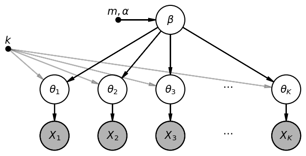
In this problem, we’ll use a Bayesian hierarchical model to model the number of failures, \(X_i\), for each of \(n\) power plant pumps1. Consider the following Gamma-Poisson model, \[ \begin{align*} \beta &\sim \text{Gamma}(m,\alpha)\\ \theta_i \mid \beta & \sim \text{Gamma}(k,\beta), \;\; i=1,\ldots,n\\ X_i \mid \theta_i & \sim \text{Poisson}(\theta_i), \;\; i=1,\ldots,n, \end{align*} \] where the \(\theta_i\) are independent of each other and represent the rate of failures for each power plant pump. The \(\beta\) and \(\theta_i\) are unknown parameters, and \(m\), \(\alpha\), and \(k\) are fixed and known.
We’d like to infer the parameters \(\beta\) and the \(\theta\) from the data \(X\). That is, we’d like to sample from the posterior distribution \(\mathbb{P}(\beta, \theta \mid X)\) using Gibbs sampling. This entails deriving the posterior of each parameter, conditioned on the data and all the other parameters.
6.2.1 (a)
Drawing the Graphical Model
Draw a graphical model which best represents the specified Gamma-Poisson model.
Answer
We have the following graphical model:
6.2.2 (b)
Finding the Conditional Distribution of \(\beta\)
Let’s start with \(\beta\). Derive \(\mathbb{P}(\beta \mid \theta_1, \ldots, \theta_n, X_1, \ldots, X_n)\).
Answer
\(\text{Gamma}\left(nk + m, \alpha + \sum_{i=1}^n \theta_i \right)\)
\[ \begin{align*} \mathbb{P}(\beta \mid \theta_1, \ldots, \theta_n, X_1, \ldots, X_n) &= \mathbb{P}(\beta \mid \theta_1, \ldots, \theta_n) \\ &= \frac{\mathbb{P}(\beta) \prod_{i=1}^{n} \mathbb{P}(\theta_i \mid \beta)}{\int_0^\infty \mathbb{P}(b) \prod_{i=1}^{n} \mathbb{P}(\theta_i \mid b) \, db}\\ & \propto_\beta \beta^{m-1} e^{-\alpha \beta} \prod_{i=1}^n \beta^k e^{-\beta \theta_i}\\ &\propto_\beta \beta^{nk + m - 1}e^{-(\alpha + \sum_{i=1}^{n} \theta_i) \beta} \\ & \propto_\beta \text{Gamma}(nk+m, \alpha + \sum_{i=1}^{n} \theta_i). \end{align*} \]
Here’s the same derivation one step at a time. Our goal is \[ p(\beta \mid \theta_1, \ldots, \theta_n, X_1, \ldots, X_n). \] In other words, given all the pump failure rates \(\theta_i\) and observed failures \(X_i\), what is the distribution of \(\beta\)?
Start with the graphical model from part (a), where white nodes are unknown parameters and gray nodes are observed data. Notice that \(\beta\) influences the \(\theta_i\), which then influence the \(X_i\). Once we know all the \(\theta_i\), observing the \(X_i\) provides no additional information about \(\beta\). Therefore: \[ \boxed{p(\beta \mid \theta, X) = p(\beta \mid \theta)} \] This is an example of conditional independence. It’s the Markov blanket idea from the Bayes net representation review in my CS 188 Discussion 07 notes: \(\beta\)’s children are \(\theta_1, \ldots, \theta_n\), and those children have no other random parents, so the \(\theta_i\)’s form \(\beta\)’s Markov blanket.
Next, apply Bayes’ rule: \[ p(\beta \mid \theta_1, \ldots, \theta_n) \propto p(\beta)\, p(\theta_1, \ldots, \theta_n \mid \beta). \] Since the \(\theta_i\) are conditionally independent given \(\beta\), we can write: \[ \boxed{p(\beta \mid \theta) \propto p(\beta) \prod_{i=1}^n p(\theta_i \mid \beta)} \] This is just the familiar Bayesian relationship \[ \text{Posterior} \propto \text{Prior} \times \text{Likelihood}, \] where \(p(\beta)\) is our prior, and the product of the Gamma densities is our likelihood for \(\beta\).
Now substitute the Gamma distributions. Recall that the Gamma density, using the shape-rate parameterization, is \[ \text{Gamma}(a, b): \quad f(u) = \frac{b^a}{\Gamma(a)} u^{a-1} e^{-bu}. \] Our prior is \(\beta \sim \text{Gamma}(m, \alpha)\), so \[ p(\beta) \propto \beta^{m-1} e^{-\alpha\beta}. \] Next, because \(\theta_i \mid \beta \sim \text{Gamma}(k, \beta)\): \[ p(\theta_i \mid \beta) = \frac{\beta^k}{\Gamma(k)} \theta_i^{k-1} e^{-\beta\theta_i}. \] We’re deriving the distribution of \(\beta\), so we can discard factors that don’t depend on \(\beta\) (here \(\frac{1}{\Gamma(k)}\) and \(\theta_i^{k-1}\)). Notice that \(\beta^k\) stays, because \(\beta\) is the rate parameter of this Gamma. That leaves \[ p(\theta_i \mid \beta) \propto_\beta \beta^k e^{-\beta\theta_i}. \] Putting everything together: \[ p(\beta \mid \theta) \propto_\beta \beta^{m-1} e^{-\alpha\beta} \prod_{i=1}^n \beta^k e^{-\beta\theta_i}. \]
Simplify the product in two pieces. First, the powers of \(\beta\): \[ \beta^{m-1} \prod_{i=1}^n \beta^k = \beta^{m-1+nk}. \] Second, the exponential terms: \[ e^{-\alpha\beta} \prod_{i=1}^n e^{-\beta\theta_i} = e^{-\beta\left(\alpha + \sum_{i=1}^n \theta_i\right)}. \] Combining: \[ \boxed{p(\beta \mid \theta) \propto \beta^{nk+m-1} e^{-\left(\alpha + \sum_{i=1}^n \theta_i\right)\beta}} \]
Finally, recognize the Gamma distribution by comparing with the Gamma kernel: \[ \underbrace{u^{a-1} e^{-bu}}_{\text{Gamma kernel}} \] We can identify: \[ \begin{align*} a - 1 &= nk + m - 1 \quad \Longrightarrow \quad a = nk + m, \\ b &= \alpha + \sum_{i=1}^n \theta_i. \end{align*} \] Therefore: \[ \boxed{\beta \mid \theta, X \sim \text{Gamma}\left(nk + m,\ \alpha + \sum_{i=1}^n \theta_i\right)} \]
6.2.3 (c)
(Optional) Finding the Conditional Distribution of \(\theta_i\)
Next, we’ll look at each \(\theta_i\). Derive \(\mathbb{P}(\theta_i \mid \beta, \theta_1, \ldots, \theta_{i-1}, \theta_{i+1}, \ldots, \theta_n, X_1, \ldots, X_n)\)
Answer
\(\text{Gamma}\left(X_i + k, \beta + 1\right)\)
\[ \begin{align*} &\mathbb{P}(\theta_i \mid \beta, \theta_1, \ldots, \theta_{i-1}, \theta_{i+1}, \ldots, \theta_n, X_1, \ldots, X_n) \\ &\quad = \mathbb{P}(\theta_i \mid \beta, X_i)\\ &\quad = \frac{\mathbb{P}(\theta_i, \beta, X_i)}{\mathbb{P}(\beta, X_i)} \\ &\quad = \frac{\mathbb{P}( X_i \mid \theta_i, \beta) \mathbb{P}(\theta_i \mid \beta) \mathbb{P}(\beta)}{\mathbb{P}(\beta, X_i)} \\ &\quad = \frac{\mathbb{P}(\beta)\mathbb{P}(\theta_i \mid \beta) \mathbb{P}(X_i \mid \beta, \theta_i)}{\mathbb{P}(\beta) \int_0^\infty \mathbb{P}(u \mid \beta) \mathbb{P}(X_i \mid \beta, u) \, du} \\ &\quad = \frac{\mathbb{P}(\theta_i \mid \beta) \mathbb{P}(X_i \mid \beta, \theta_i)}{\int_0^\infty \mathbb{P}(u \mid \beta) \mathbb{P}(X_i \mid \beta, u) \, du} \\ &\quad \propto_{\theta_i} \theta_i^{k-1} e^{-\beta \theta_i} \theta_i^{X_i} e^{-\theta_i} \\ &\quad \propto_{\theta_i} \theta_i^{X_i + k -1} e^{-(\beta + 1) \theta_i} \\ &\quad \propto_{\theta_i} \text{Gamma}(X_i + k, \beta + 1). \end{align*} \]
The first equality is the same Markov blanket argument: \(\theta_i\)’s parent is \(\beta\), its only child is \(X_i\), and \(X_i\) has no other parents, so \(\{\beta, X_i\}\) is \(\theta_i\)’s Markov blanket and the other \(\theta_j\)’s and \(X_j\)’s drop out. This is exactly the “resample \(X\) from \(P(X \mid \text{Markov blanket}(X))\)” step in the Gibbs sampling review from my CS 188 Discussion 07 notes. For practice recognizing what Gibbs sampling can and can’t produce, see CS 188 Discussion 07, Bayes’ Nets Sampling (e).
6.2.4 (d)
Implementing a Gibbs Sampler in Pseudocode
Using the posterior distributions you derived in the last two parts, write out the algorithm for the Gibbs Sampler.
Answer
Initialize \(\beta^{(0)} \sim \text{Gamma}(m, \alpha)\) and \(\theta_i^{(0)} \mid \beta = \beta^{(0)} \sim \text{Gamma}(k, \beta^{(0)})\) for all \(i\).
For \(t=1, \ldots, T\) for some large stopping time \(T\):
Start with \((\beta^{(t-1)}, \theta_1^{(t-1)}, \ldots, \theta_n^{(t-1)})\) from the previous iteration.
Sample \(\beta^{(t)}\) according to \[ \begin{align*} \beta^{(t)} &\sim \mathbb{P}(\beta \mid \theta_1 = \theta_1^{(t-1)}, \ldots, \theta_n=\theta_n^{(t-1)}) \\ &= \text{Gamma}(nk+m, \alpha + \sum_{i=1}^{n} \theta^{(t-1)}_i) \end{align*} \]
Sample the \(\theta_i^{(t)}\) in parallel according to \[ \begin{align*} \theta_i^{(t)} \sim \mathbb{P}(\theta_i \mid \beta = \beta^{(t)}, X_i = x_i) = \text{Gamma}(x_i + k, \beta^{(t)} + 1) \end{align*} \] Note that we are allowed to sample \(\theta_i^{(t)}\) in parallel because each \(\theta_i\)’s updates do not depend on each other.
E I George, U E Makov, and A F M Smith. Conjugate likelihood distributions. Scandinavian Journal of Statistics, 20:147–156, 1993.↩︎